


Learning The Houdini Spirit
Last updated | 12/28/2025
As a 3D Generalist with fascination in tool development and programming, I have been slowly transitioning into a Technical Artist. My background in 3D started with a passion for character development. After a decade later, the idea of being a Technical Artist seems to align really well with where I am going as a 3D artist. So, I've decided to transition into this role, not saying it will be easy, but given my interests I believe this would be a step in the right direction. So where should I start? I have heard that Houdini is a great tool for a Technical Artist. Especially for tooling and pipeline solutions. In this blog I wanted to share my first Houdini project.
To get started, obviously I needed Houdini. Thankfully Houdini has an apprentice version, which is free and restricted in a few areas such as commercial use, file export, rendering watermarks, but for the most part the tools to learn Houdini's environment are available. To get started though, we can at-least learn my way around Houdini, and stay in its environment.
Getting to know the interface is the first step of learning a new software. Which may also prove as a challenge. I think once I get comfortable navigating the UI in Houdini, I'll be able to get my feet grounded in this environment and pick out the different fruits here. The nodes panel is the most intimidating, and I'm sure many share this feeling. Not only in Houdini, but other DCCs as well.
NOTE: The image gallery sequences from left to right. So the top left image would be referred to as image 1. Next image is image 2, and so on.
Basics
To pan around the viewport in Houdini we press+hold alt and click+hold the middle-mouse button(scroller).
To rotate we press+hold "alt" click+hold the left-mouse button.
To zoom in and out we press+hold "alt" with click+hold right-mouse button.
Viewport Operations
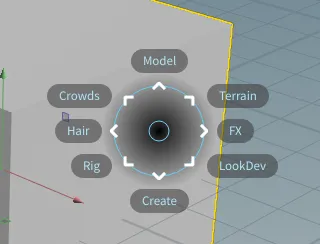
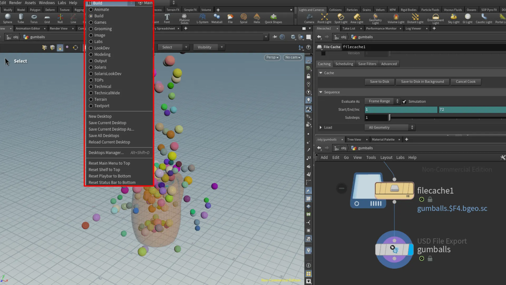
We can perform different operations in the viewport by pressing C.
This displays a pie menu shown below.
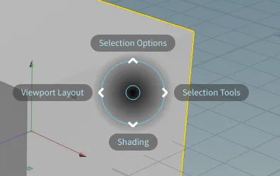
We can change display type in the viewport by pressing V.
When adding a new object in the viewport, we press the C key and select create, then we can add a box for an example. You can also press
First project: SideFX H21 Foundations
Surface Operators(SOPs) | Modeling a cup
For my first project in Houdini, I am following along an introduction to Houdini tutorial by Robert Magee on Side FX. This project includes modeling a cup in Houdini, creating a distributor for spheres to scatter on the distributed points, simulation, lighting, rendering, materials and textures. It's a great intro to Houdini tutorial, and easy to follow along, but I suppose that also depends on your familiarity of the 3D fundamentals.
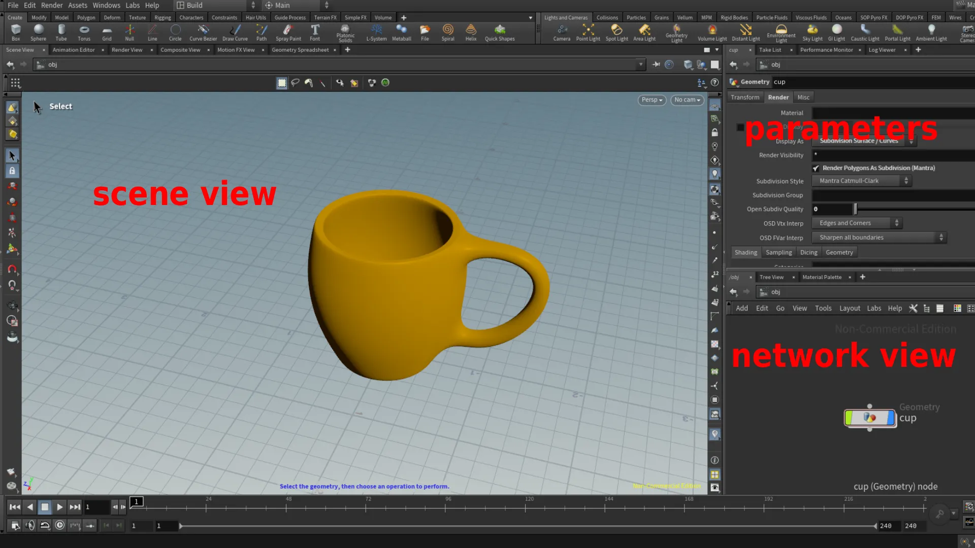
Below shows the different node levels of the cup I modeled following along the tutorial. Modeling in Houdini is the same as other 3D DCCs, in terms of terminology and functionality of the operations. The biggest strength here in Houdini is its "non-destructive" or "collapsing" procedural work-flow. Essentially, everything in Houdini is procedural, which gives it a huge advantage over other 3D packages. You can see the node tree on the right side, which makes up the cup model.
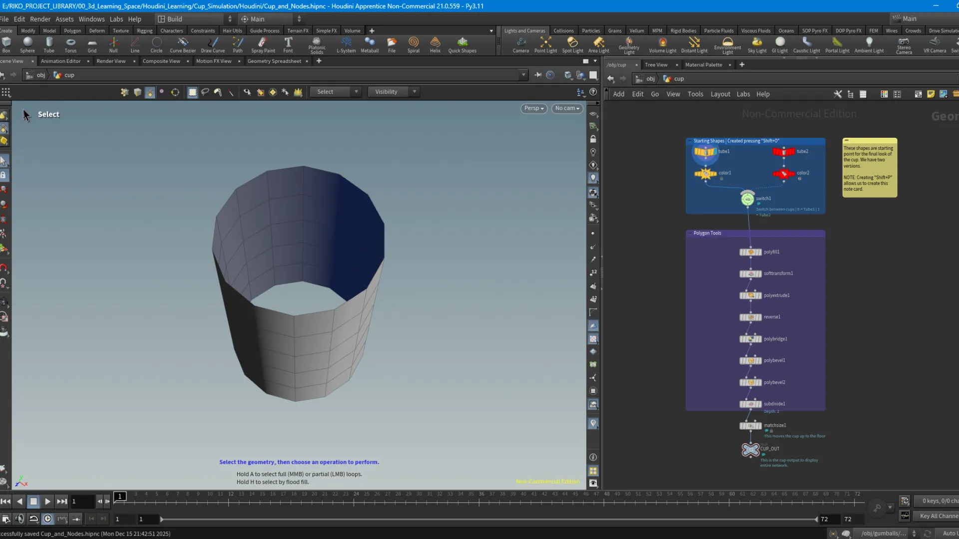
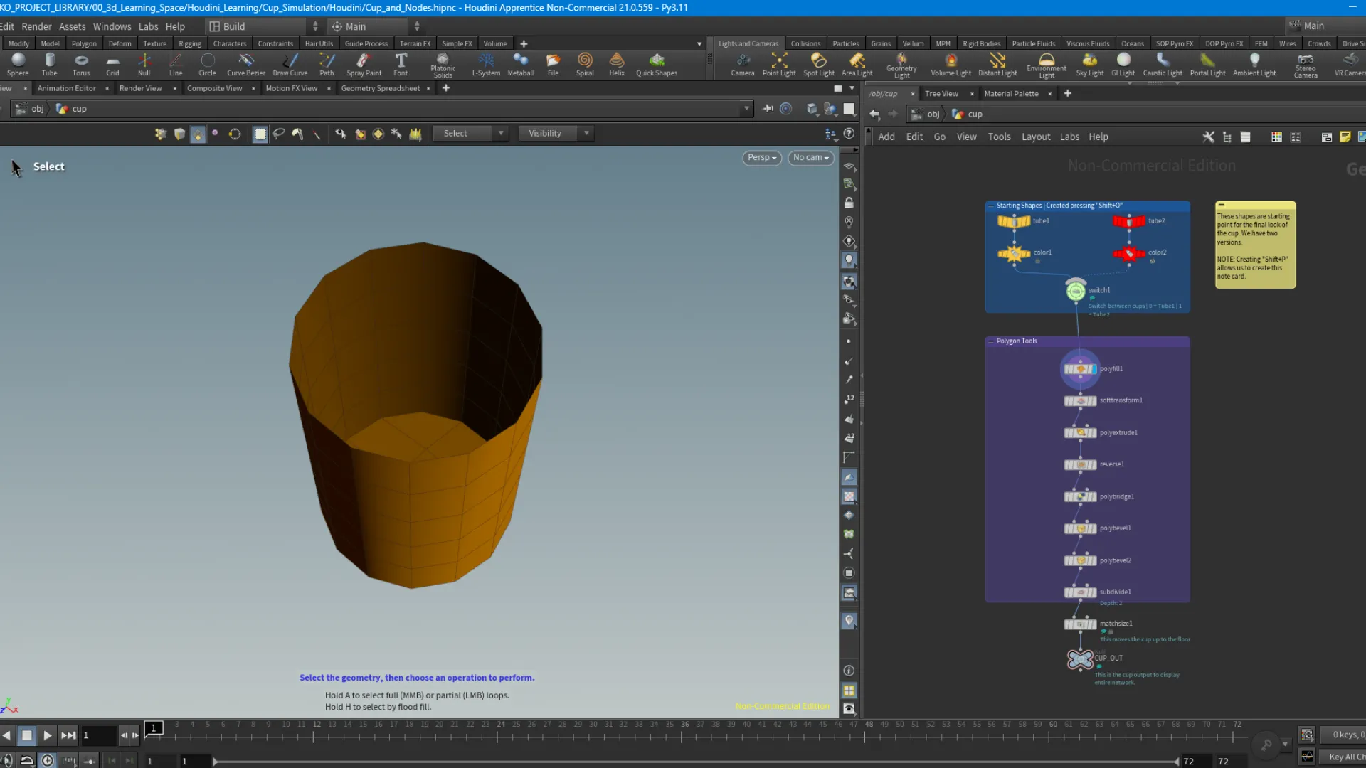
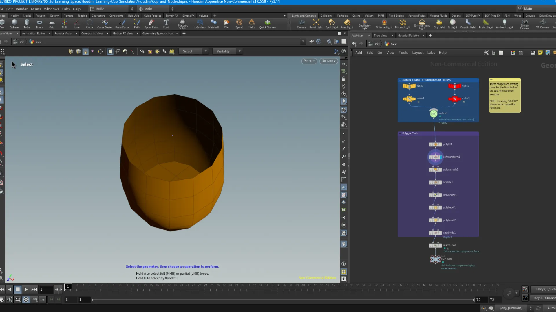
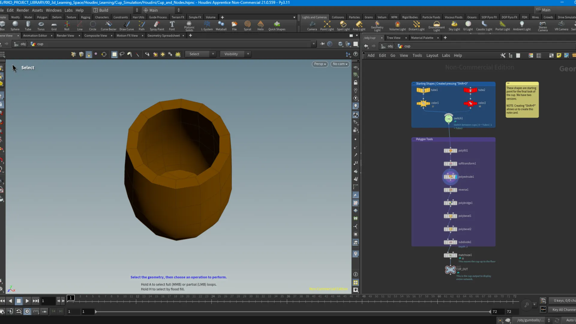
Working With The Networks View
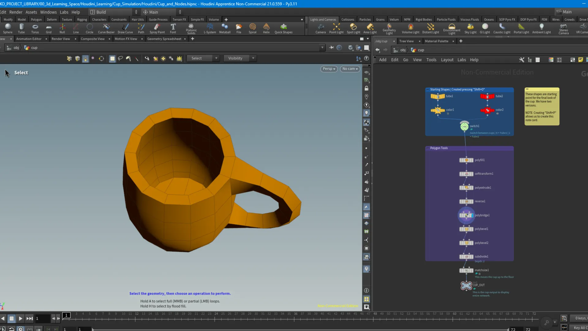
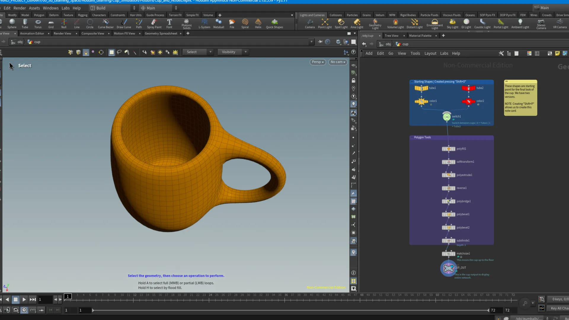
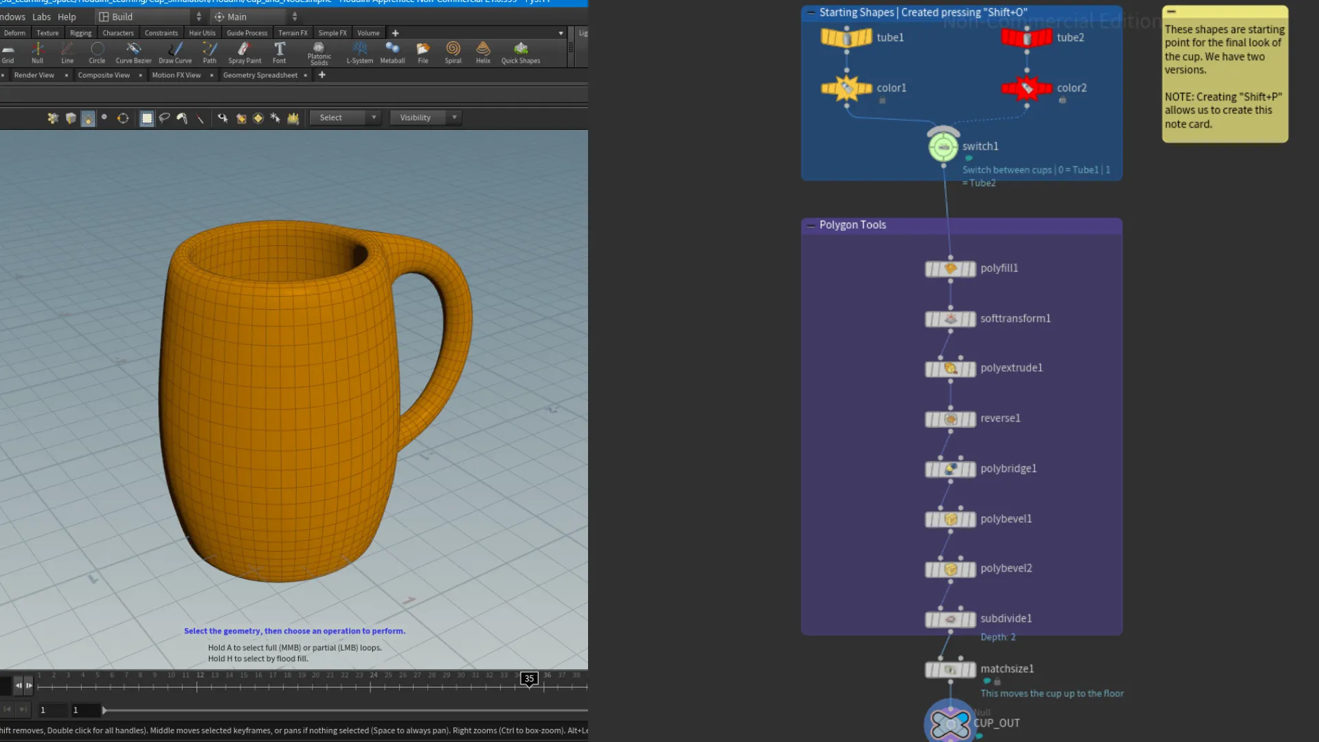
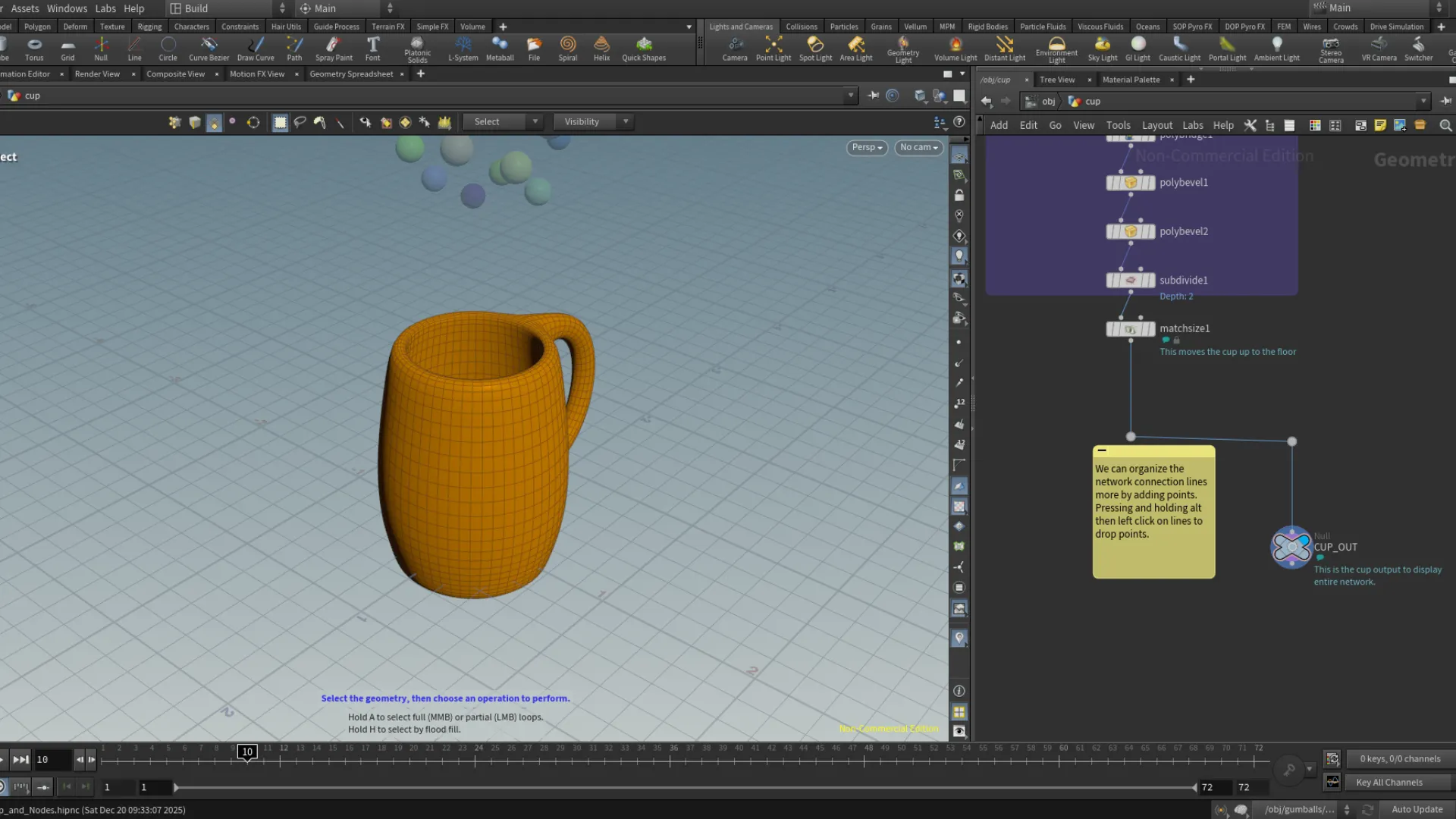
This is the final build of the cup and the node tree representing its different stages of development. For the most part, modeling the cup was a familiar process with standard operations. The learning curve here, again, is getting familiar with the UI; the different parameters and fields. The tutorial also showed us how we can work within the network view. We can group nodes together by creating a layout frame around the selected by pressing Shift + O. We can also create a notes frame with Shift + P within the Networks View panel. Another neat way to make notes on a specific node is to hover over the node, then on the left side there is an i icon. Clicking on this will open a window with information regarding the node. At the bottom of it there is a Node Comment section. Once adding a comment, we have to enable it to show next to the node. There are a few Display Flags on a node, and these can be used for debugging as well. At the bottom of the node tree for the cup, we added a Null node. This is used as a global display for the entire node tree. The way I am understanding this is, if we continue to build on this cup, we can set Null nodes at different points of our node tree and through these nodes we can display certain groups of the node tree, which is very helpful.
To organize any nodes that are misaligned a certain direction, we can press and hold A + left-mouse hold, then drag to the direction you want to align the selected nodes. Use Y + left-mouse hold to enable scissor and cut connections. J + left-mouse hold to connect node(s). You can click and drag over multiple nodes to the direction they should connect. Finally, you can organize the network even more by adding connection points on the connection lines between nodes by pressing alt hold + left-mouse click on the lines.

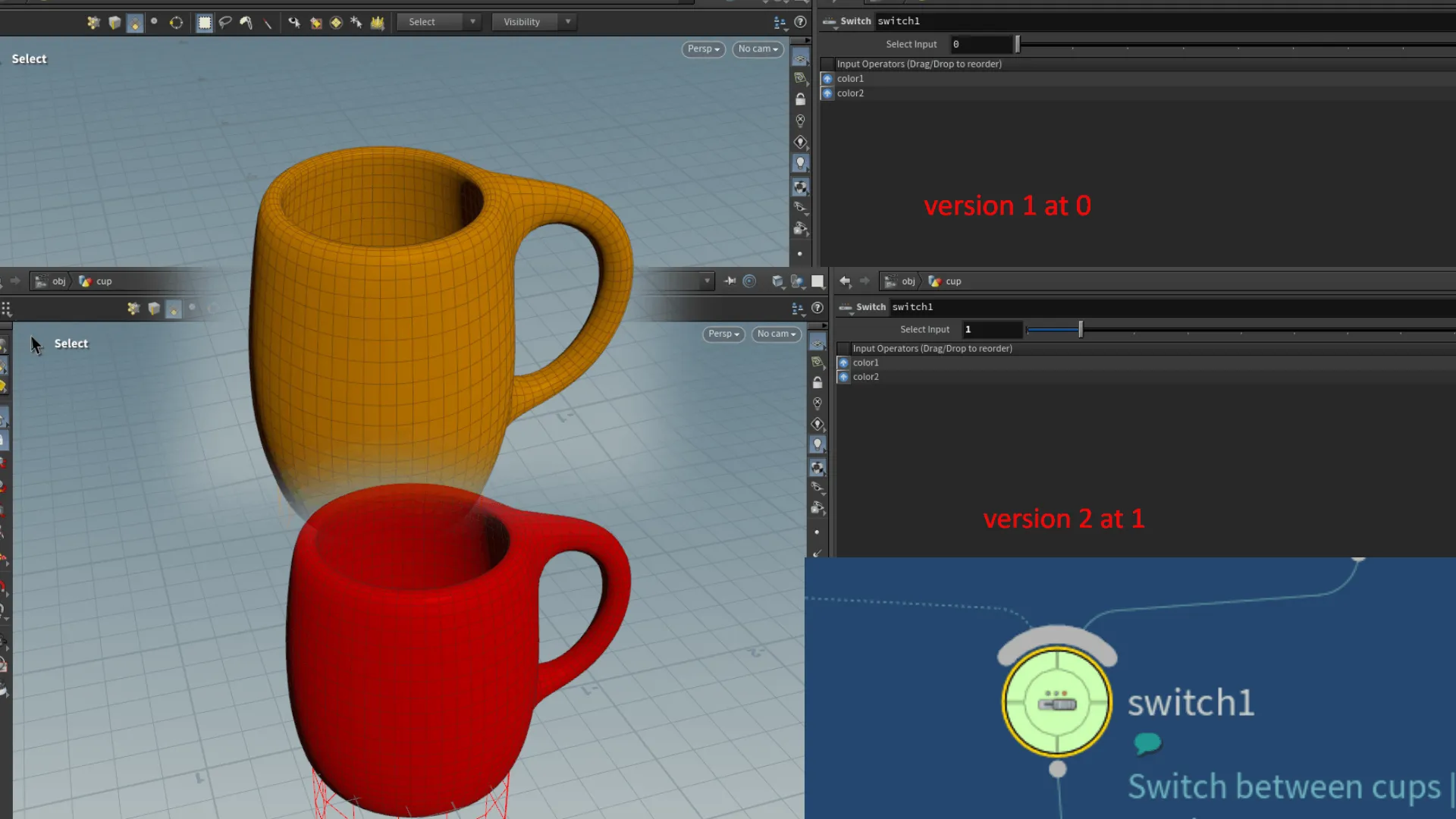
In this I was shown how we can use the Switch node to have a variation of the cup model running through the model's node tree. Using a switch node, we can switch from one to the other through incrementing integers with index 0 being the first version, 1 being the second and so on.
Seeing the node tree is one thing, but the process is another. Above the node panel by default is the parameters panel. Here we have the different attributes belonging to a certain operation or function, where we can tweak and edit. As a beginner in Houdini, the parameters can also look a bit intimidating, especially sitting on top of the nodes panel. These are technical things that I think I will wrap my head around in time as I continue learning Houdini. This goes for any software really.
The nice thing is I have some experience working in similar environments such as Blender's geometry nodes panel.Panels such as the properties/attributes will always have a plethora of parameters to get familiar with, so I think this area of the UI is something I'll also get used to in time.
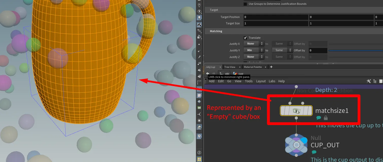
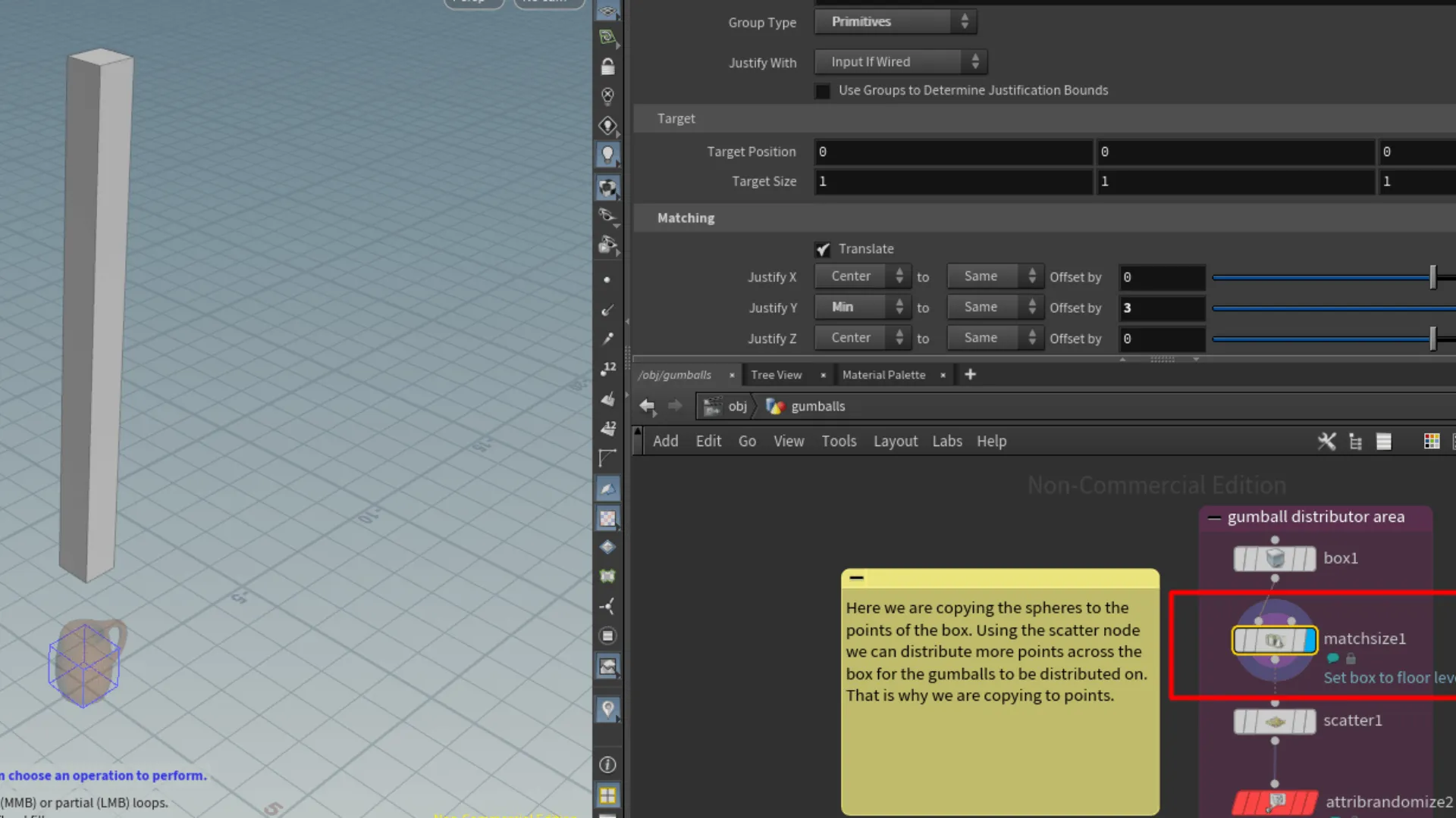
Aside from the standard operations I did to block-out the geometry into a shape of a cup, the thing that stood out to me the most here is the Match Size node. When we want to add a new object to the viewport, we select the object we want either from the header or pressing the C key. We can then press Enter and the object will be placed at the origin. However the object ends up sitting centered with half of it below the grid plane. So to make the object sit on top of the grid plane, we use the Match Size node.
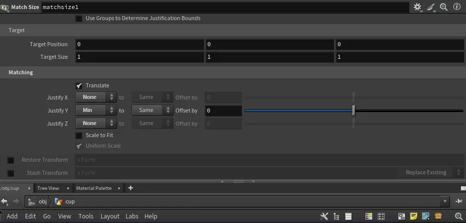
In the Match Size node we set the JustifyY parameter to Min, and we can also set X and Z to None. Doing this will place the object it is applied to at the top of the grid plane.
Making gumballs
The second element to this project was distributing spheres across a box object, using the scatter node to distribute the points. First we needed an object to scatter the points over. In the H21 Foundations tutorial, we used a box and increased the height. Here we are also using the Match Size node to set the box at the top of the grid level. Then we offset it in the Y axes to 3 so that it floats above the cup. Then we had to use the Copy to Points node to instance the sphere at each point. We also want to make sure to check the Pack and Instance field. I think this enables each sphere to be treated as a primitive/geometry. This is a similar operation to Blender's instance node and using the realize instance node to register instances as a geometry. Below shows the starting setup for the gumballs.
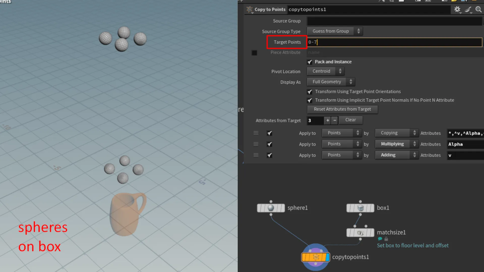
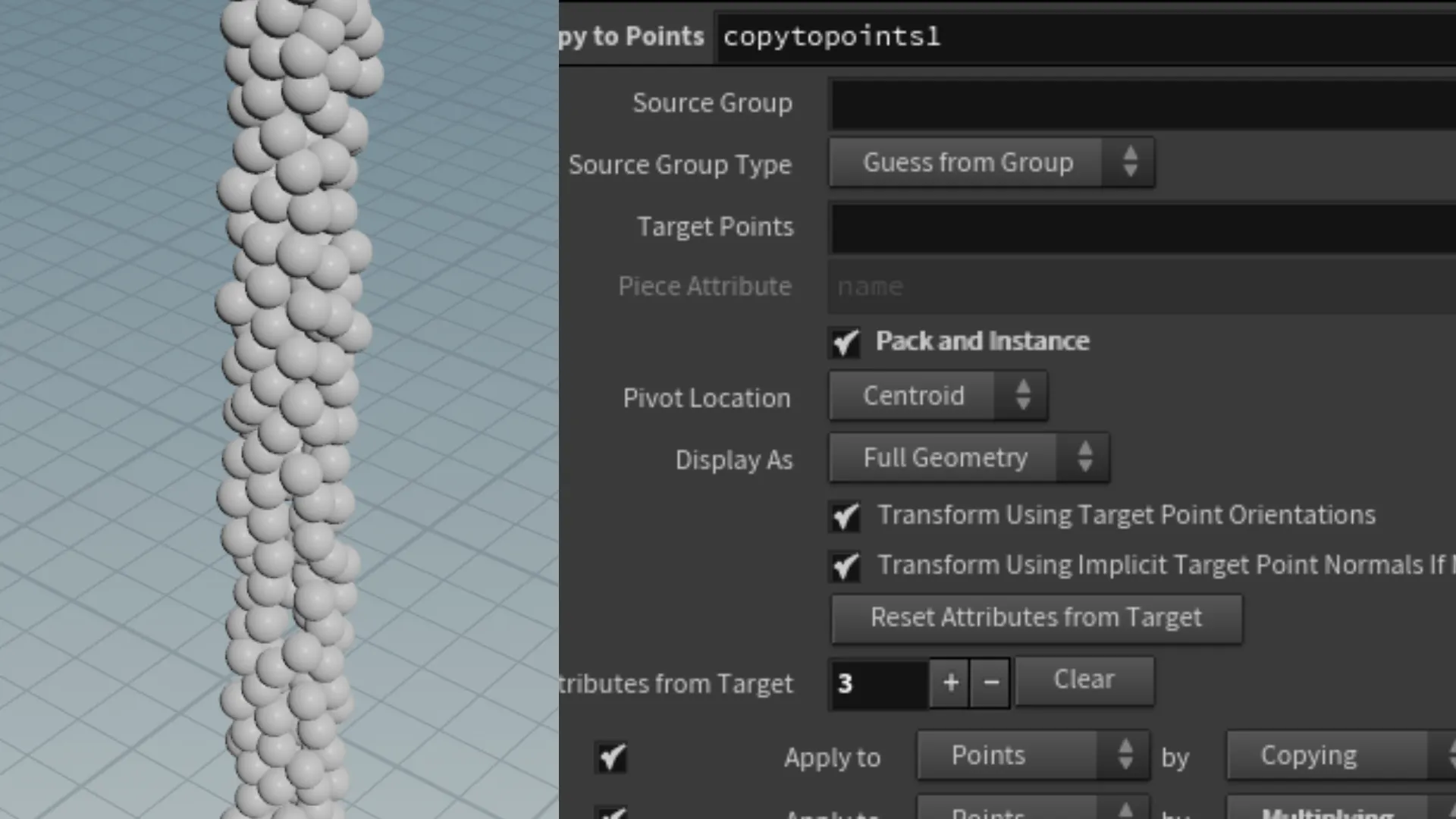
In the screenshot of the parameters panel, there is a Target Points field, which includes the value range from 0-7. We actually set this to 0, or leave the field empty, so that all points are considered. Leaving the range here, would result in only the points from index 0-7 to have the sphere instanced over.
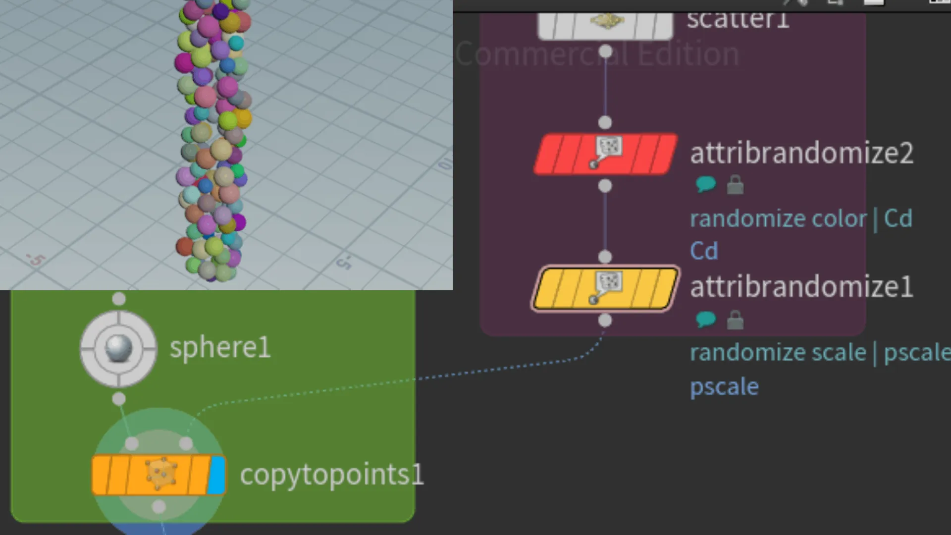
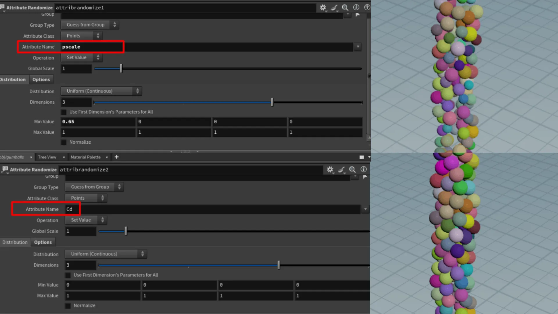
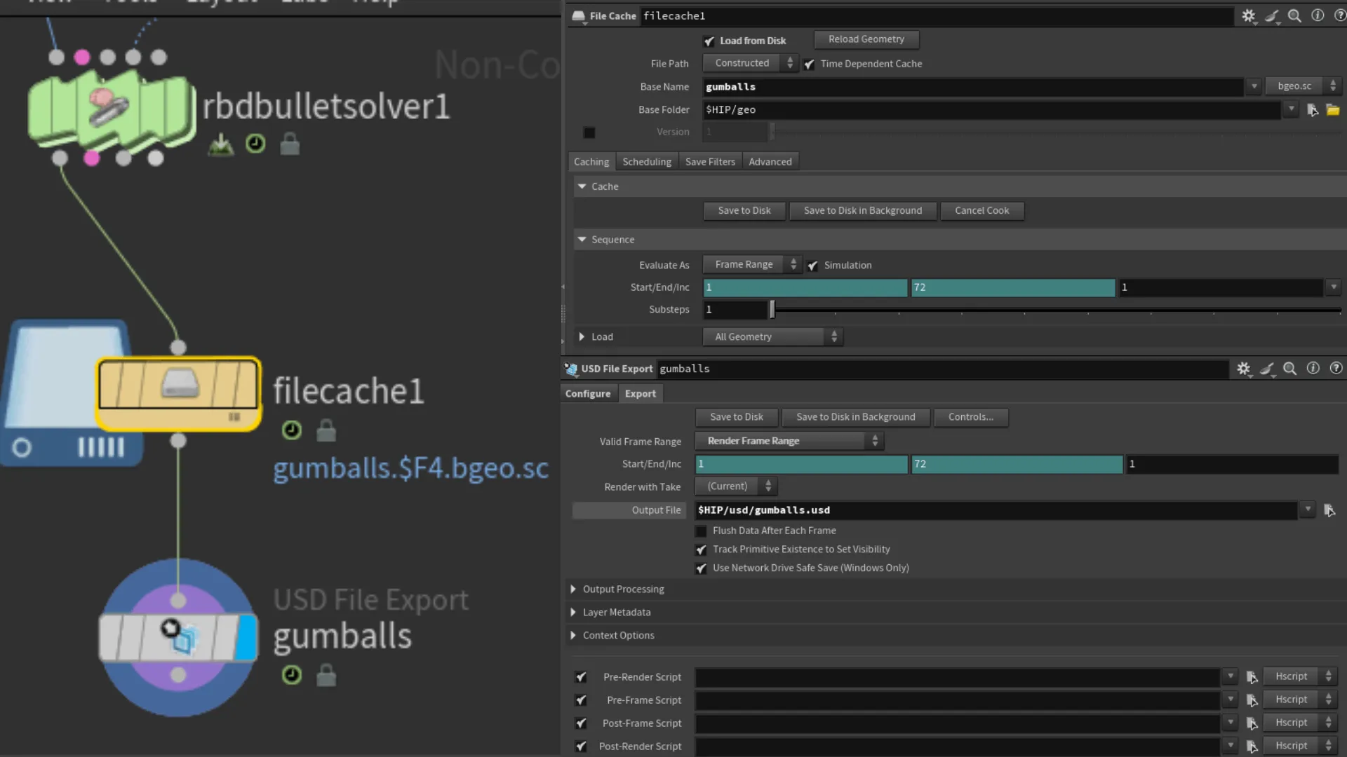
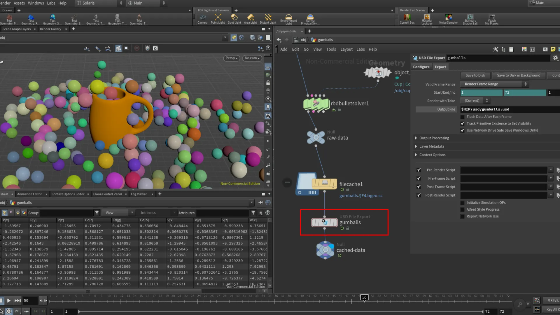
Another great node to work with in these sort of scenarios is the Randomize Attribute node. Through this node we can randomize the colors of each sphere and also randomize the scale of each sphere. This tutorial introduced me to two attribute names or call tags I suppose we could call it. "Cd" and "pscale". Last few steps for this was adding the simulation node called RBD Button Solver. We then added a File Cache node to cache the simulation, and a USD File Export node to export the gumballs as a USD file.
Solaris Desktop
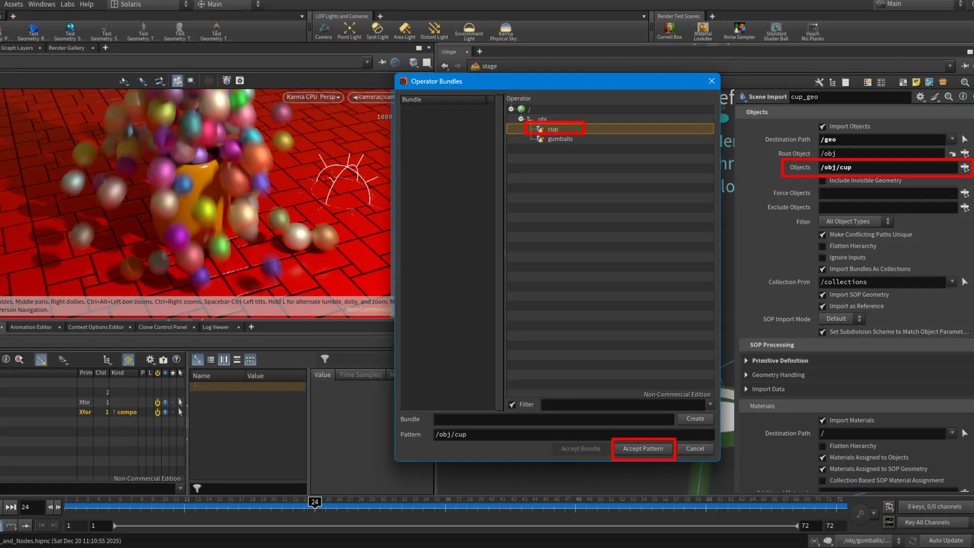
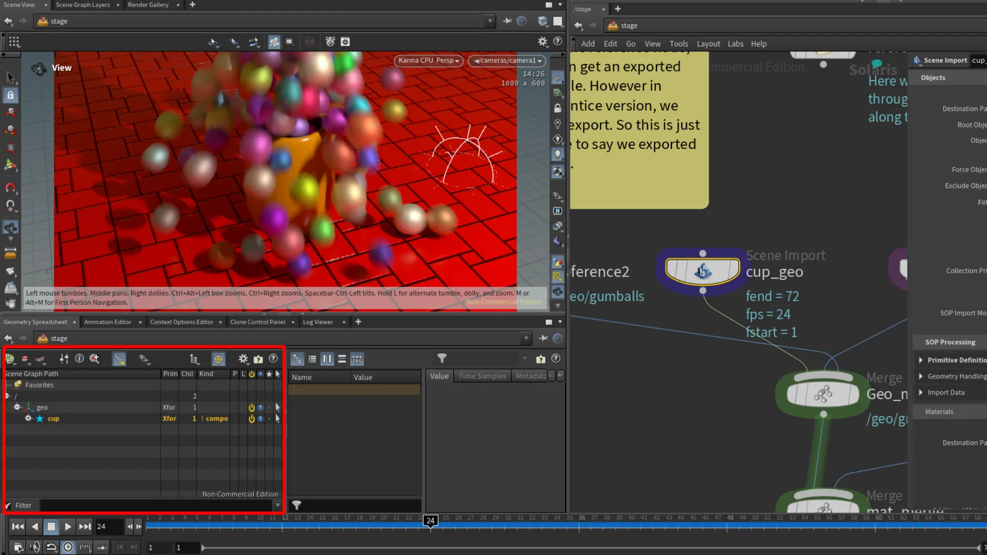
In the fourth part of the H21 Foundations tutorial, we started working with lights and cameras. I'm going to go a bit more in depth with this section, because it was a lot for me to absorb. In this tutorial, I was introduced to the different layouts that are setups for specific scenarios, such as lighting and rendering. In Houdini, these are called Desktops. Once the Solaris desktop loads up, we have the option to switch the background color under the background tab. Press D while hovering over the Viewport to open the display menu. Again this is optional. To get started with our scene in solaris, we needed to add an Scene Import node. This allows us to import our cup object. The first image below includes the parameter settings we applied to the Scene Import node. At the right-most of the Object field, we can assign the cup object by clicking on the button and selecting the cup object, then click on the Accept Pattern. Doing this adds the object to the scene graph as well.


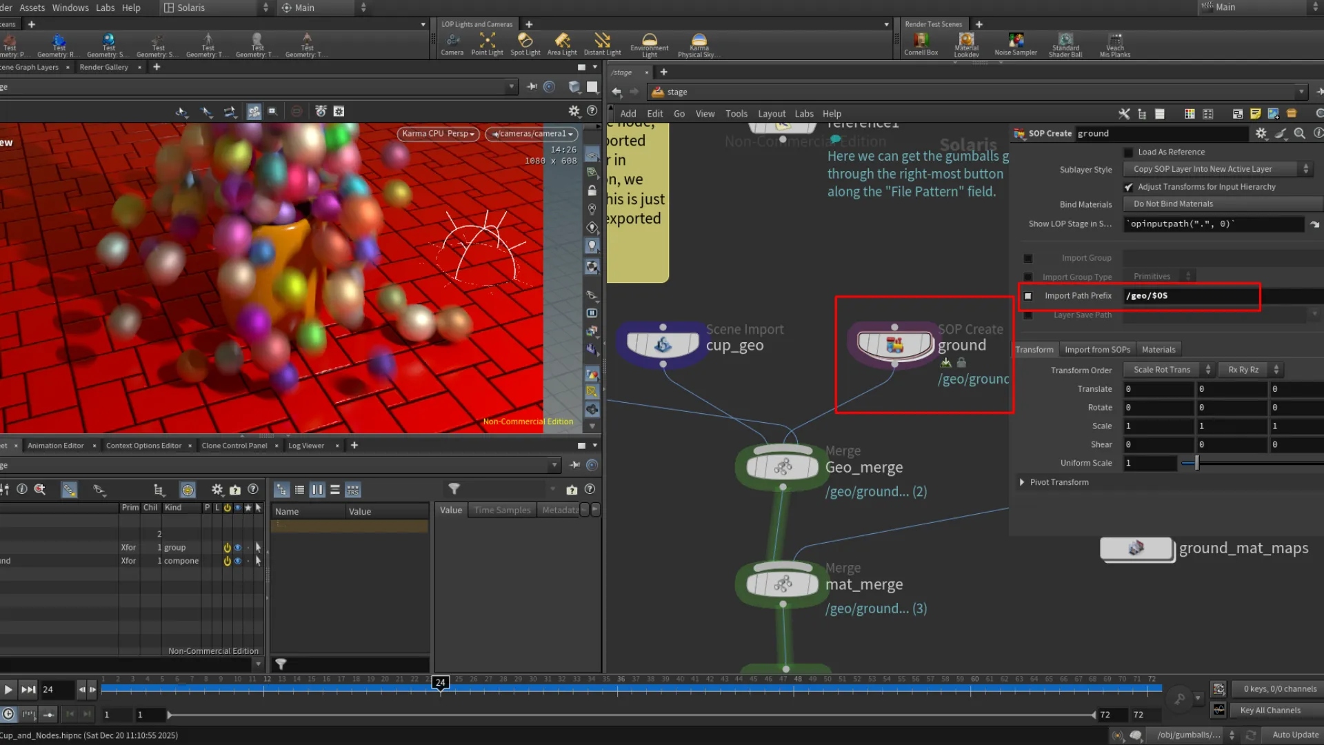
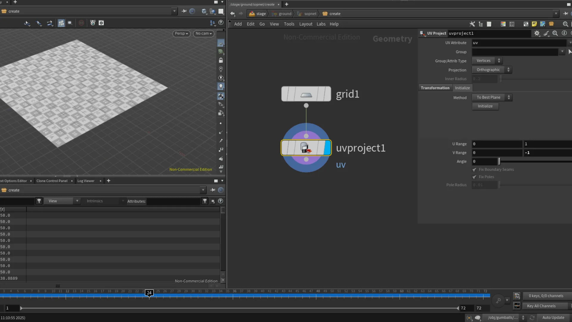
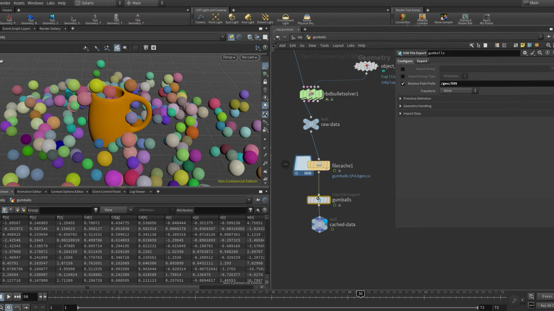
The next element we wanted to add was a plane to render the object on. Here we used the Grid node. We can add this under our geo node graph by adjust the Import Path Prefix to /geo/$OS. After adding our ground plane, we went inside its geometry level, and added a UV Project node. If the grid seems flipped, we can adjust the direction in the URange and the VRange.
Here we switch back and forth between obj and stage as the nodes we see in the nodes panel also reflect the network we are in.
NOTE: The Networks View appears empty at first here because we should be seeing the stage network, rather than the object network we were working with earlier to build the cup and simulation.
Setting Up Materials
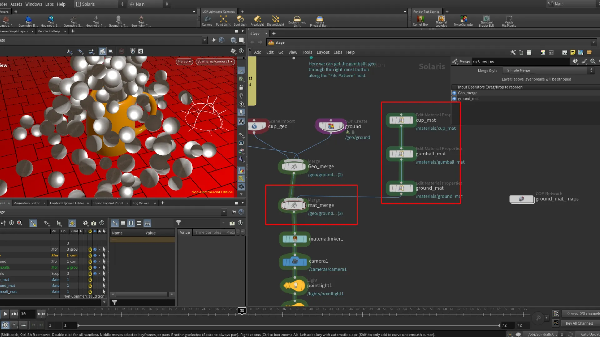
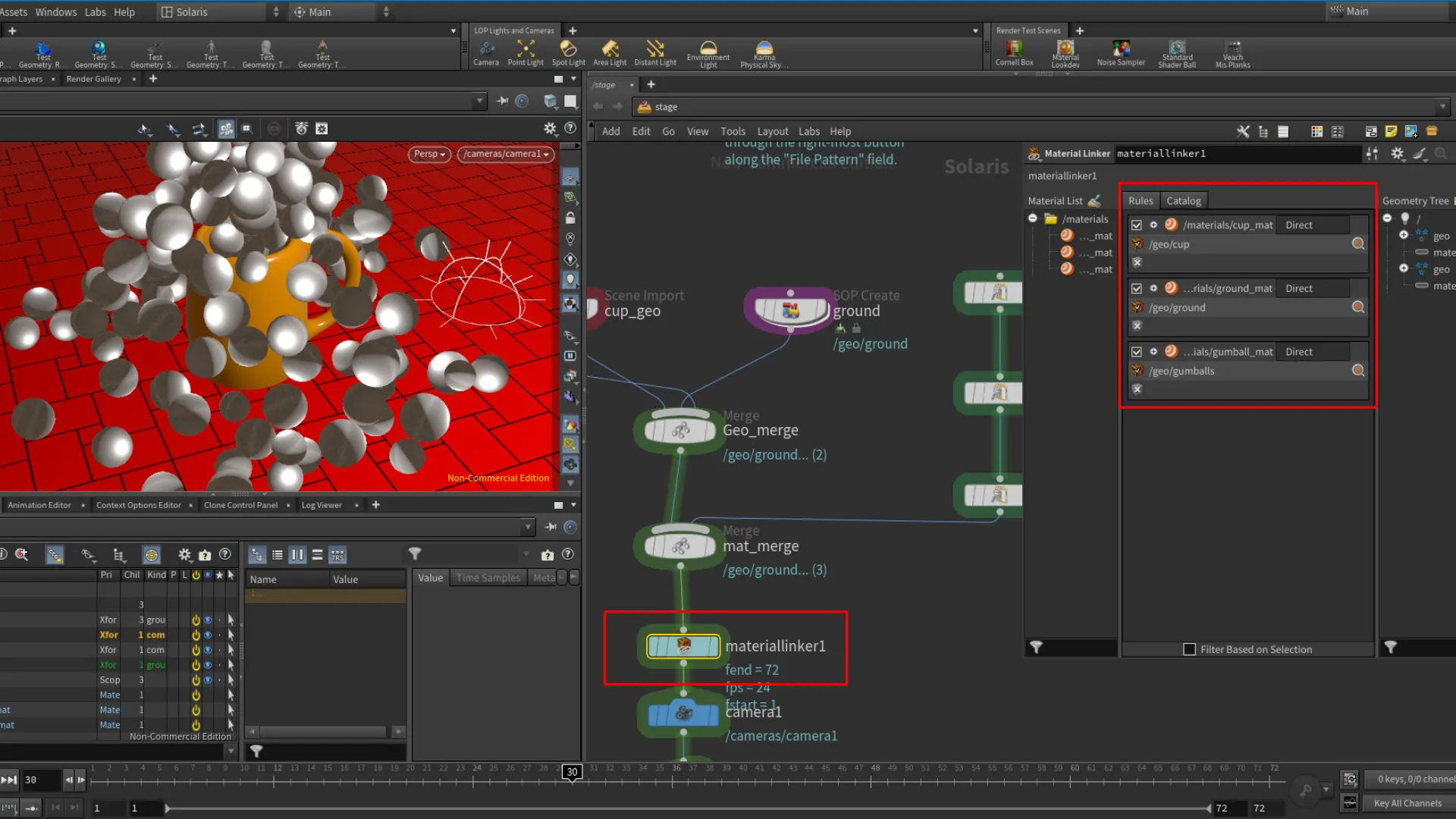
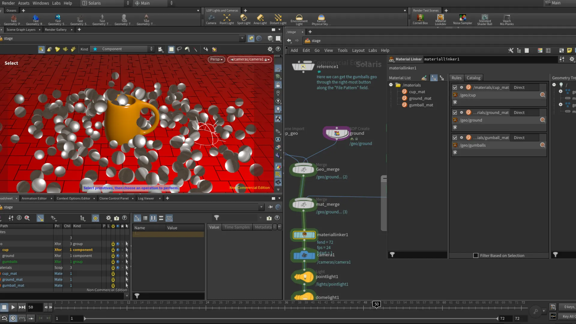
At this point we have the ground plane setup with the UV Project, we need to be back in the object level. In the Stage network and Solaris desktop, we added a Merge node and linked both the cup and ground nodes to this. This allows me to view both nodes. Now it is time to add the material nodes. Here we added a Quick Surface Material node. We need two here, so we can duplicate the first one by selecting it and pressing Alt hold + left-mouse click. To get these nodes in our network, we added another Merge node beneath the first one that merged the cup and ground nodes. We can link up the materials then the last one to the Merge node. This doesn't assign the materials to the object, but only adding it to the network tree to use. To assign the materials, we need to use a Material Linker node. With the node selected, we can drop the materials we created and merged into the Rules panel. Then we select the object from the right side of the parameters, and drop it in the geometry field of the materials. Now the materials are assigned to the objects.
This process was pretty different for me coming from Blender, 3Ds Max, and Maya.
Lights & Camera
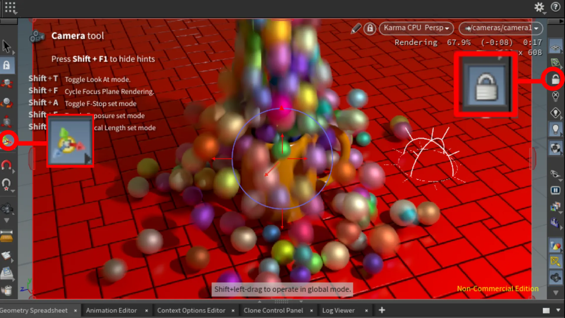
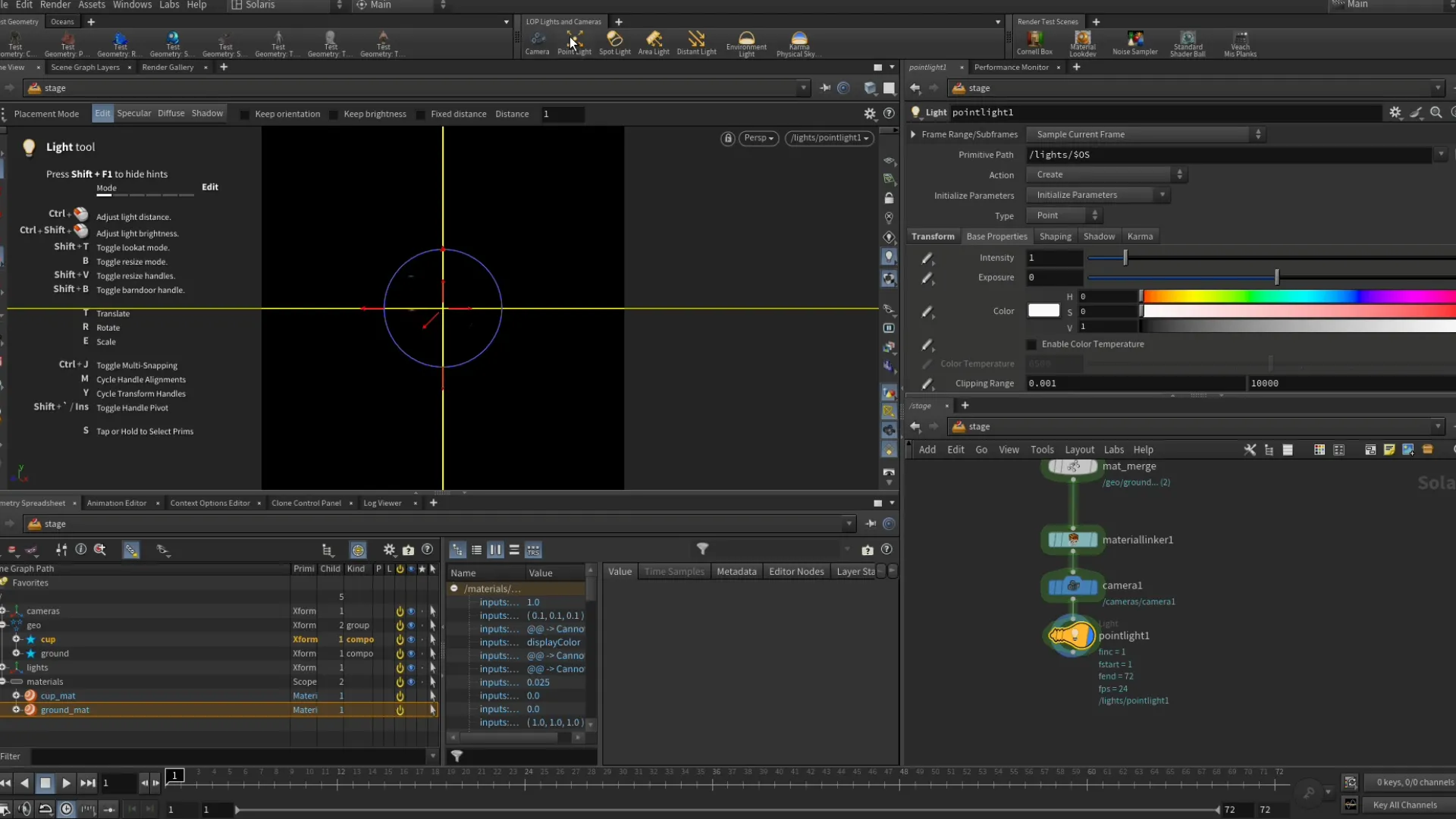
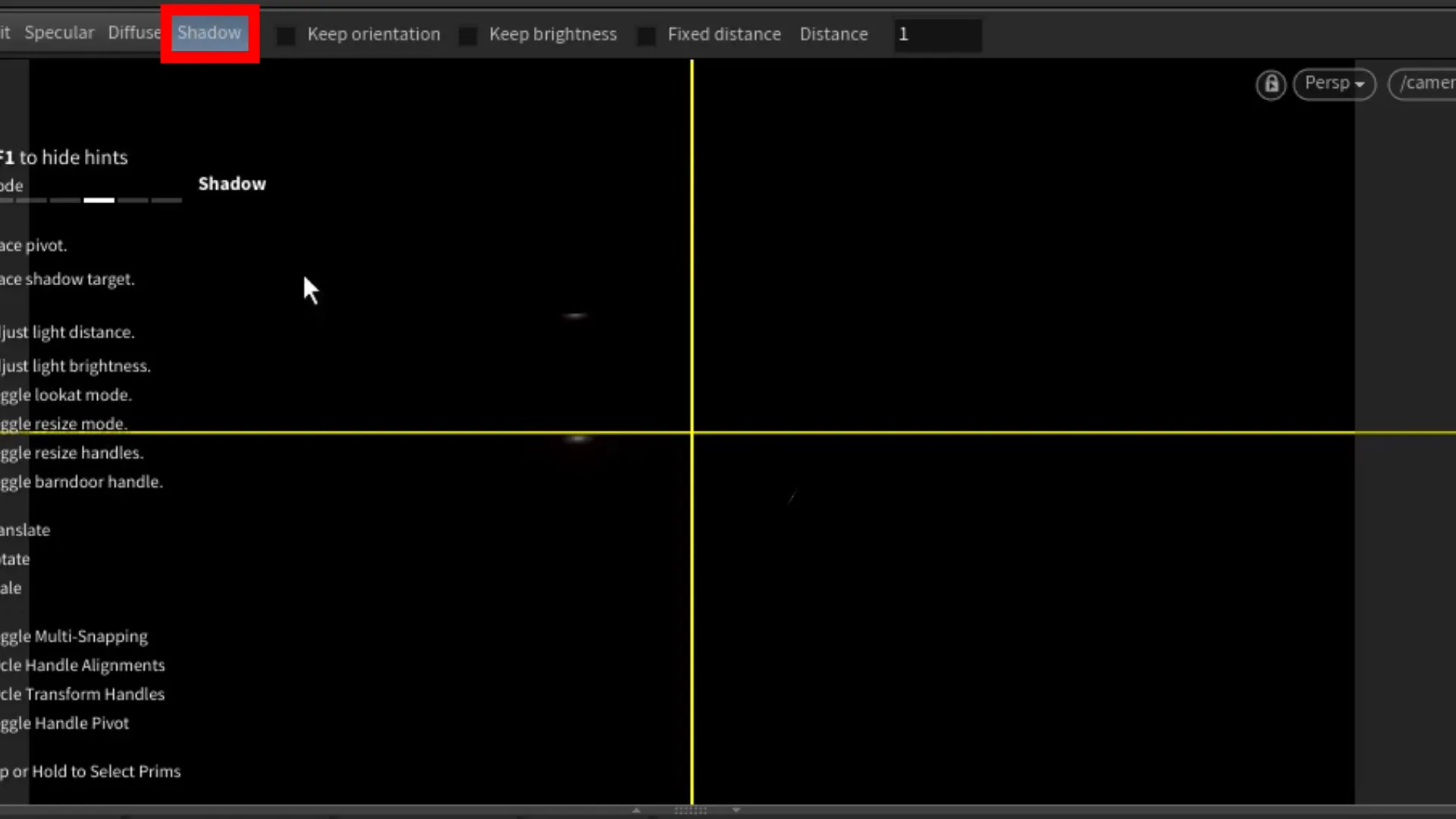
In fourth part of this course, we also added a camera and some lights. To add a camera, we can add it from the headers or press Tab, then search for Camera. When we add the camera, Houdini automatically adds it based on the perspective view position. We can move the camera around to reposition by manipulating the gizmo controls found on the Toolbar bar on the left side of the Viewport View. You can also lock the camera so that when you navigate, it'll be through the camera view. The Lock Camera tool can be found on the right Toolbar of the viewport. Next thing we added are lights. For my scene, I added a Point Light and an Dome Light to give me a global lighting. We add these the same way as everything else. Something different to me that Houdini does is when you add a light object, like the Point Light, the Viewport View will be looking through the light as it did with the camera.(See image 3) I suppose this allows us to position the light object and also setup where the light will be directing from using the Shadow mode. You can find this mode at the top-left of the viewport. Before enabling it, we can switch our view back to the camera. Which is located at the top-right corner of the viewport.
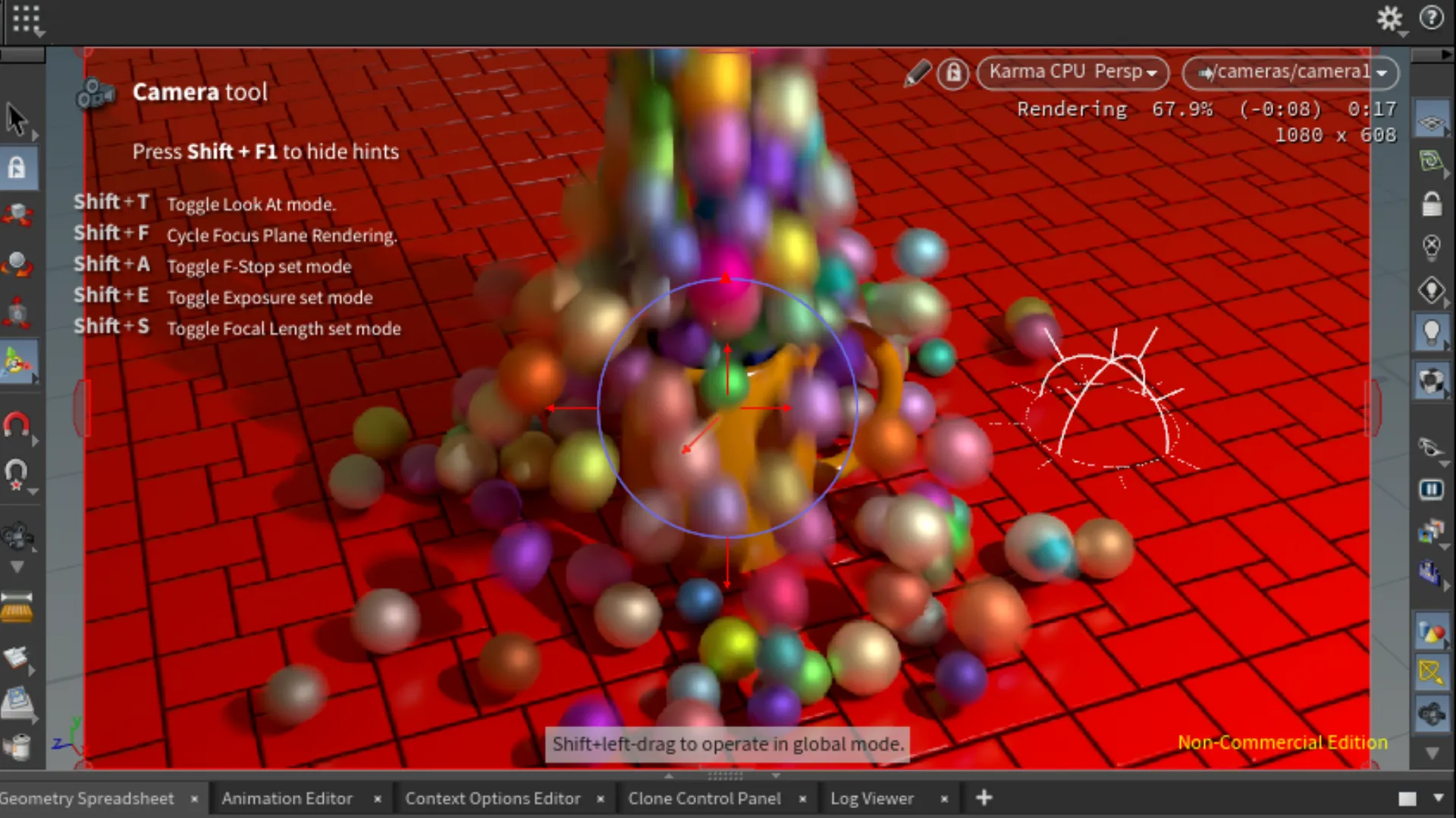
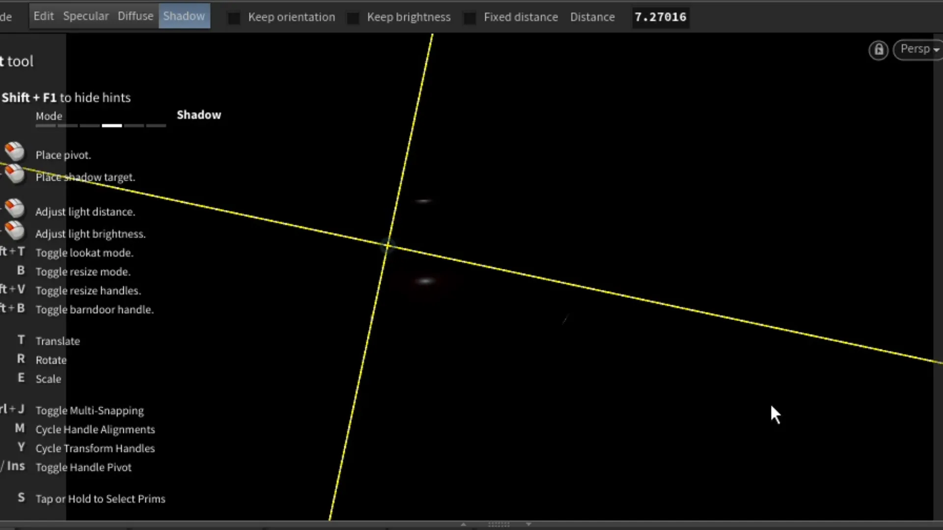
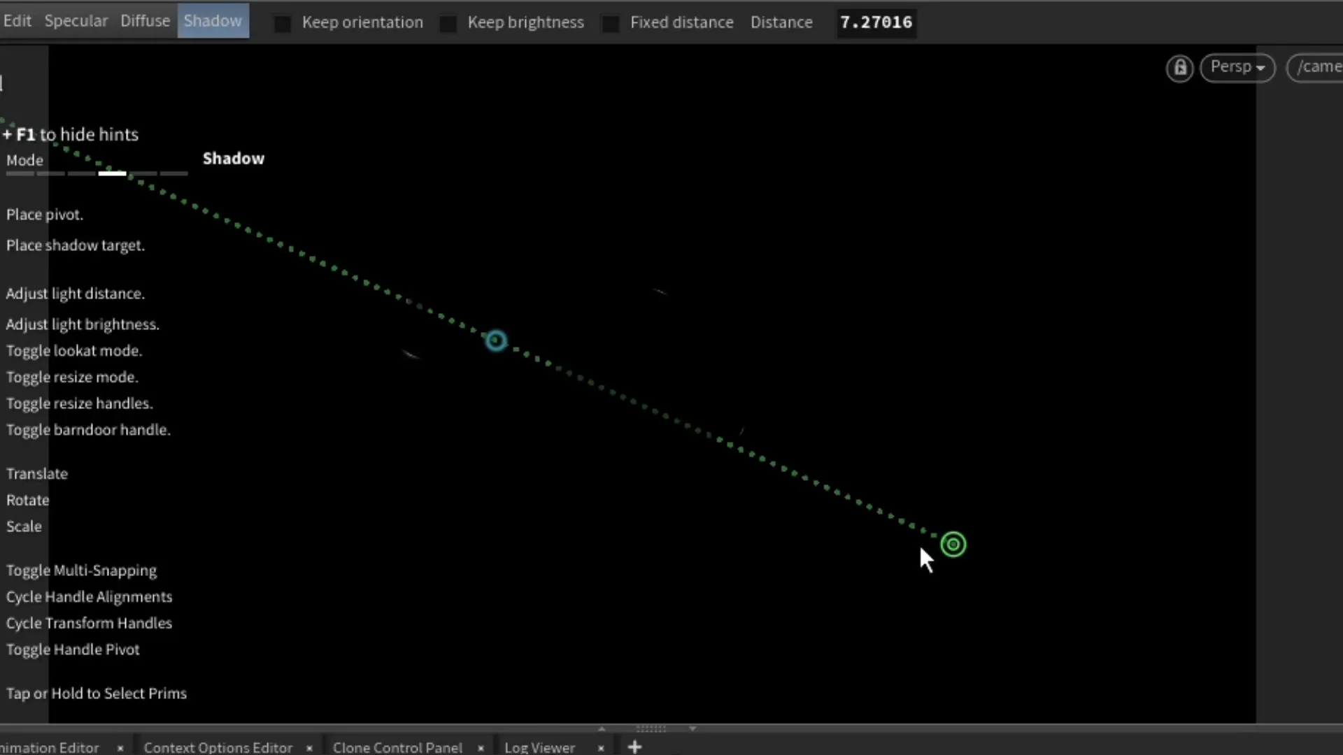
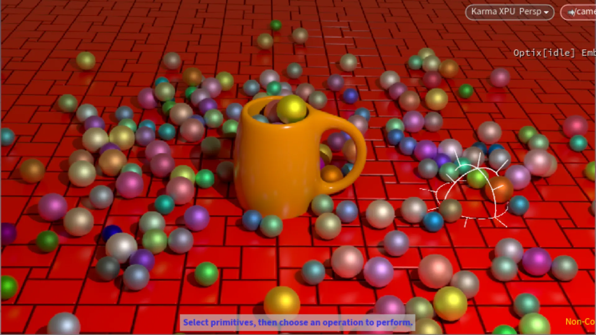
After switching back to our camera view, we can then enable the Shadow mode located at the top-left corner of the viewport.(see image 1). In this mode, we first click on the cup object, press Shift(hold) and click on the ground object, specifically the direction we want the light to be facing while focusing on the cup object. When done correctly we see something similar to images 5 & 6. When we see the distance line, we can adjust the distance of the light by pressing and holding Ctrl + left-mouse button; dragging to adjust the distance. We can adjust the intensity of the light by pressing and holding Ctrl + Shift + left-mouse button drag. Of course, we can also adjust these settings in the light's parameters.
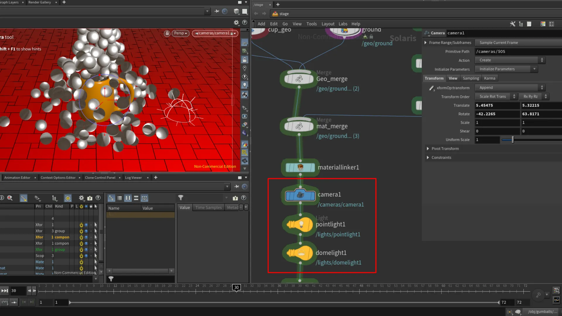
Now we should see the Camera and Light nodes under our Material Linker node.
With our camera and lights in the scene now, we can switch the Perspective View to Karma XPU or Karma CPU. The XPU version uses a combination of GPU + CPU, and the CPU version is just that.
Compositing Operators(COPs) | Texturing With Copernicus
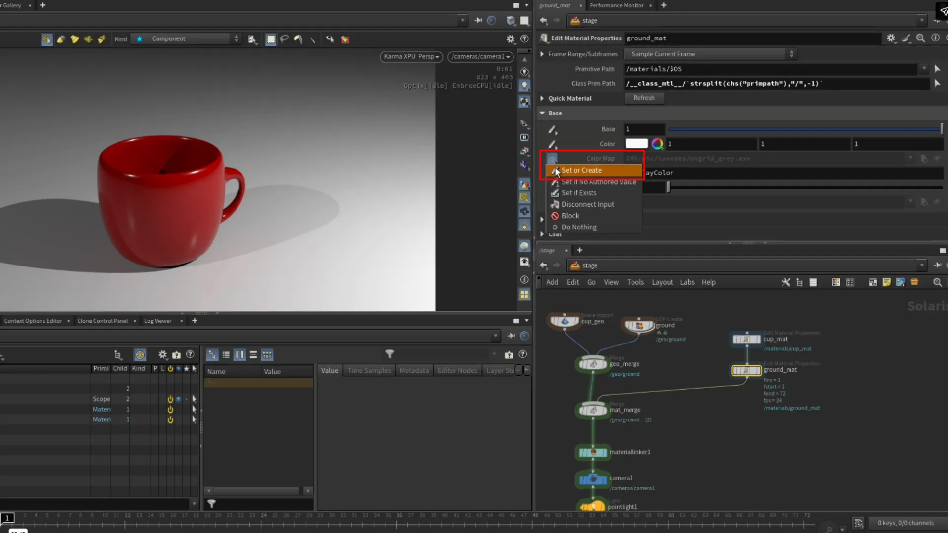
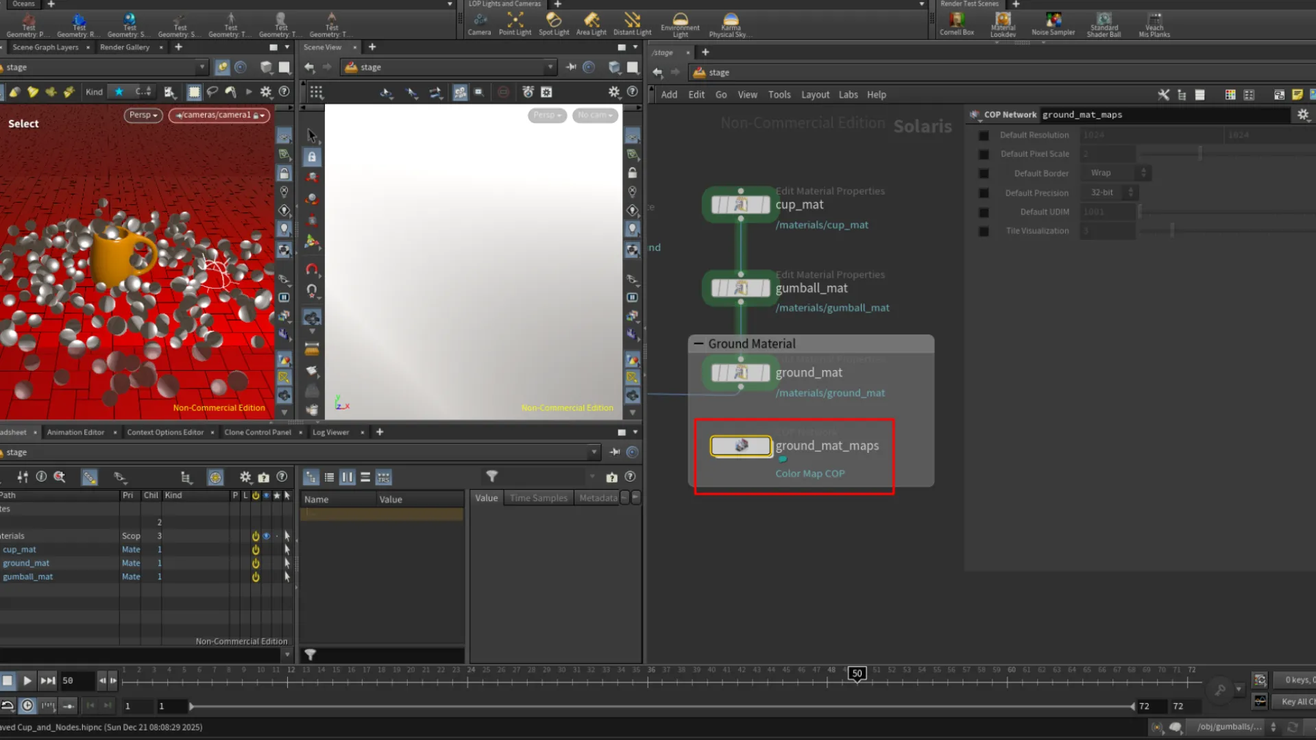
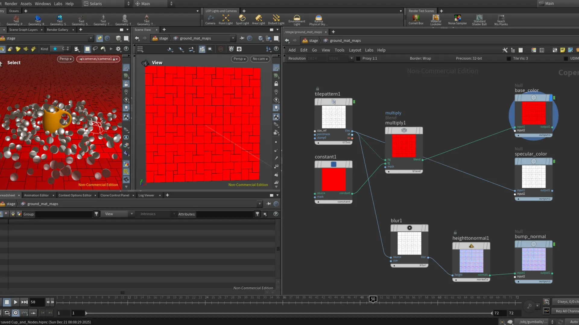
In the fifth part of this course I was shown how to work with Houdini's Copernicus system to setup textures. Also known as Compositing Operators(COPs). For this, we textured the ground plane. To create a COP Network, we have to select the material we want to work with, in this case the ground plane material, then hover over the left-most button next to one of the material properties such as the Color Map, then click on the button and Set or Create. After clicking on this, we will see a COP Network for
Adding The Gumballs
Back in the Solaris level from the compositor, with the Viewport View pin unchecked, we can switch the Network to the object level. Shown as obj. Un-pinning the viewport will allow us to see the different network we switch to. Initially, when I was following along with the tutorial, the gumballs geometry were not included in my Solaris view. So I needed to add this to the Stage I had setup my camera and lighting in. When we go back to the object level through the networks switch drop-down menu, we will see both the cup and gumballs objects. Inside the gumballs geometry level, we needed to add a USD File Export node after the File Cache node. In my version I also added a Null at the end to act as a checkpoint display node. This displays all the nodes in the network after the previous Null node.
NOTE: Adding /geo/ in the Primitive Path adds the object under "geo" in the Scene Graph Path
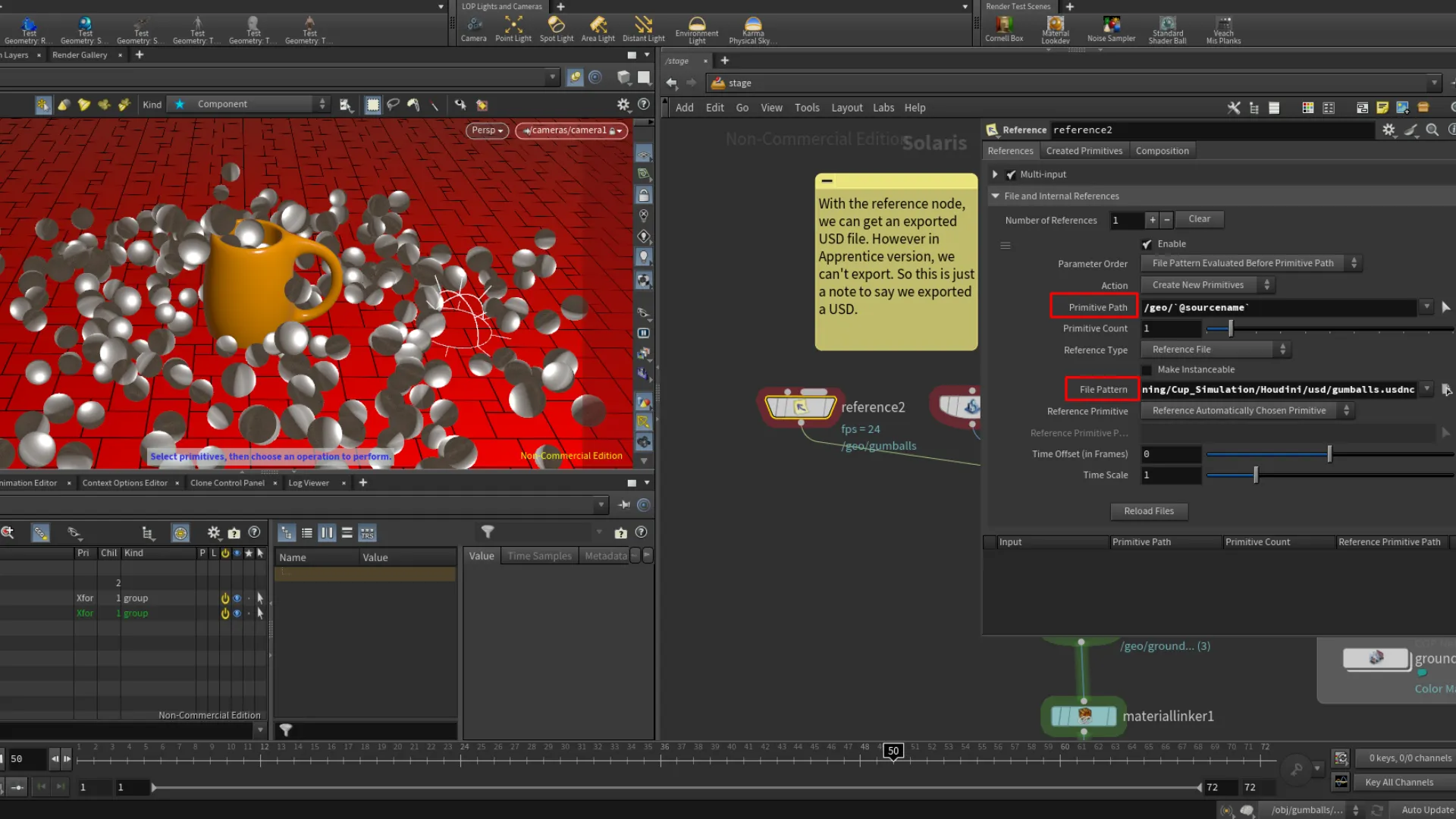
After applying the settings to the usd export node, we press on Save to Disk. This exports a cached usd of the gumballs, which we can then add it to the Stage network. Using the Reference node in the Stage network, we can get the exported usd file of our gumballs. After getting the gumballs usd, we plug the Reference node into the Merge node. We also needed to apply the gumballs material through the Material Linker following the same process as before. Dragging the material into the Rules tab, then drag the object we want to assign the material into the material. (See image 4)
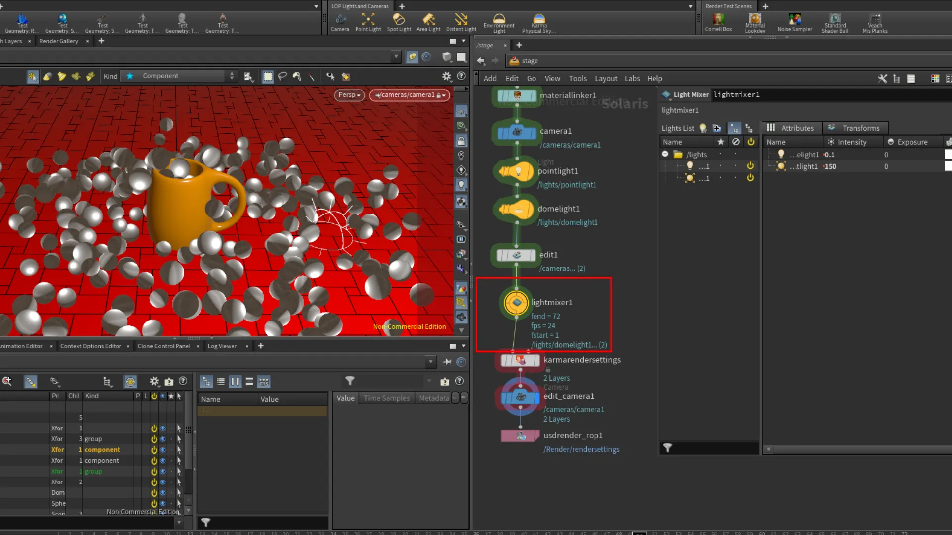
Light Mixer
We can also group the lights under one node where we can access each light in our network through a node called Light Mixer. Through the mixer, we access and adjust the light settings for all the lights in the network.
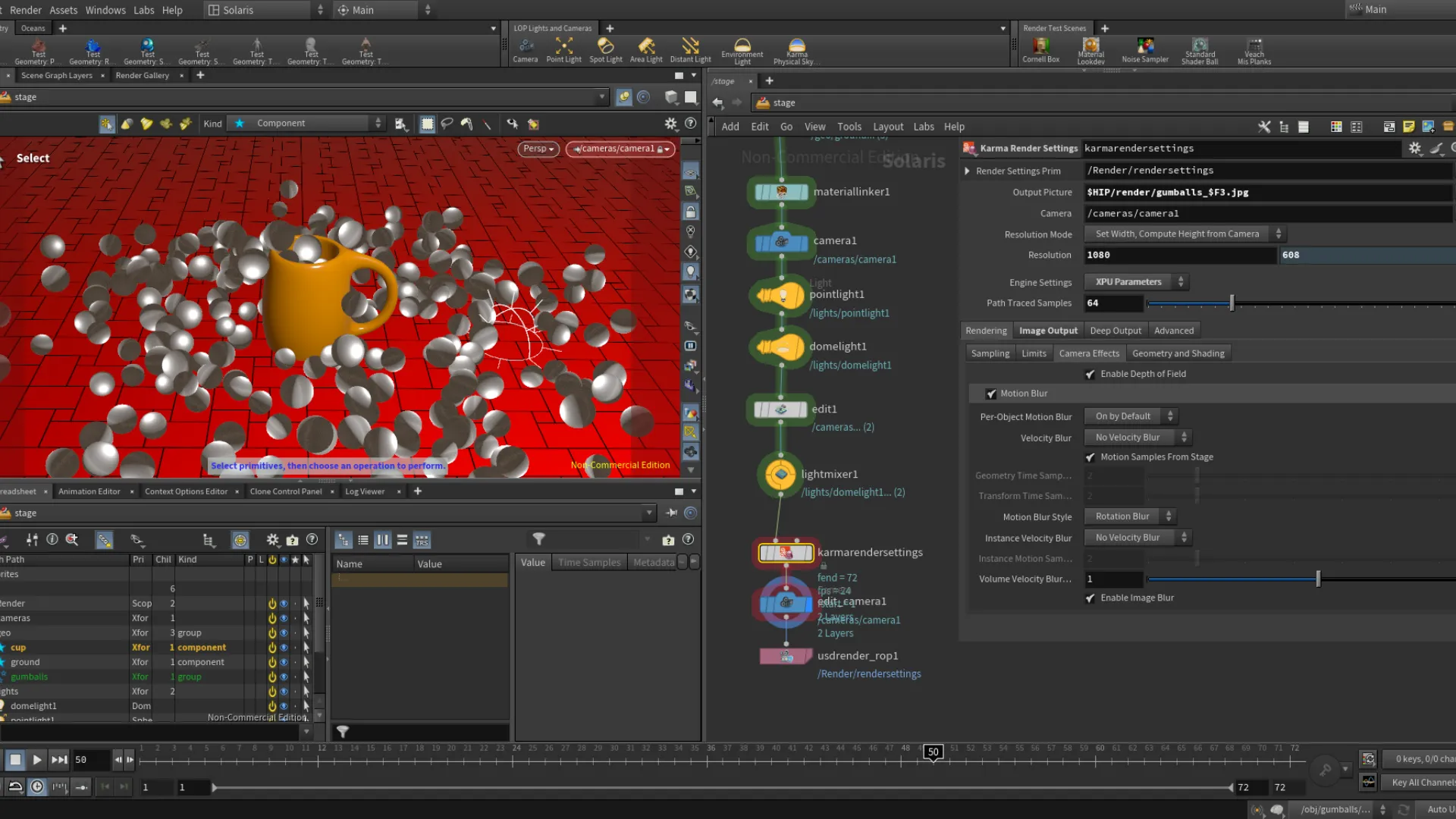
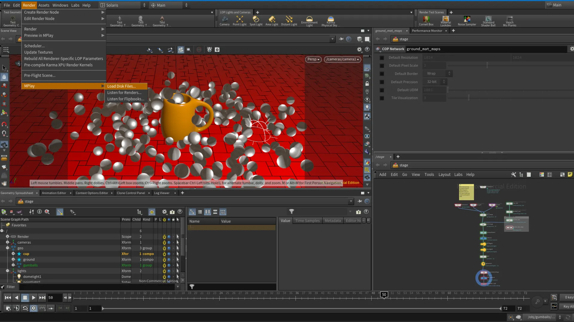
Rendering Final Shot
To setup for rendering, we use the Karma(Setup) node. The parameters are pretty self-explanatory in the Karma settings if you dealt with Render settings before in other DCCs. It just takes a while to get familiar with a different UI. After the render is finished, we can also preview the frames through Houdini's MPlay. Simply open the MPlay under the Render tab at the top menu bar, and load up the frames.
Results!
While this was a simple project, it still had its learning curves. What helped me follow along for the most part is my background in 3D. It is a different software, but has familiar functionality and terminology as other DCCs. If you made it this far in my dive into this Houdini intro, thanks for sticking around! As someone who is interested in tooling with experience in different areas of the 3D pipeline, I aim to someday be proficient in Houdini; to be able to work as a bridge between creatives and technicals. I am barely scratching the surface here, but excited to continue learning Houdini.
Course version
This is the version I had done following along with the course.
Review version
This version was done with limited guidance.
Kilelit | Blender Add-on Project
Last updated | 01/16/2026
Hey guys! This is something I'd been working on for the past six-ish years on and off in my Python learning journey. I started using Python back in 2015-ish with Maya, developing scripts focusing on rig selectors. This interest has carried on over to Blender when I picked up this software back in 2019. Since then my interest in tooling has grown exponentially. With Blender being an open-source software and community driven, it was a great source of inspiration to explore my Python interests further developing add-ons. !Kilelit is an add-on for Blender developed with the focus on automation and intuitive rendering workflow. This project went through quite a bit of changes throughout these years starting from a render button. The initial stages of the add-on was called "RenderIt", but for unique naming purposes, I changed it to "Kilelit".
“Kilel” is Ponapeian (Pohnpei, FSM) for picture or photograph, combined with “it.” Kilelit is pronounced “gil-el-it,”, or “Ki” for short.
Purchase Kilelit Github | open-source | GPL
Overview
I started this project sometime in 2020 with the idea of Blender's Cycle's render engine have similar features that other render engines include. Such as selected only rendering with a toggle, render history preview, and other render scenarios that offer an intuitive workflow in Blender. These features do not replace the built in Blender features, but the core of Kilelit is to automate these rendering scenarios which can be setup in Blender apart form it. Nevertheless, Kilelit's main purpose is to automate the rendering workflow and providing an intuitive solution for rendering scenes, history preview, and selected only renders that can be comped in post.
Render Panel
Starting off with the add-on, we have the head panel of Kilelit. The !Render panel is where the core features are located. Dealing with automating different rendering scenarios.
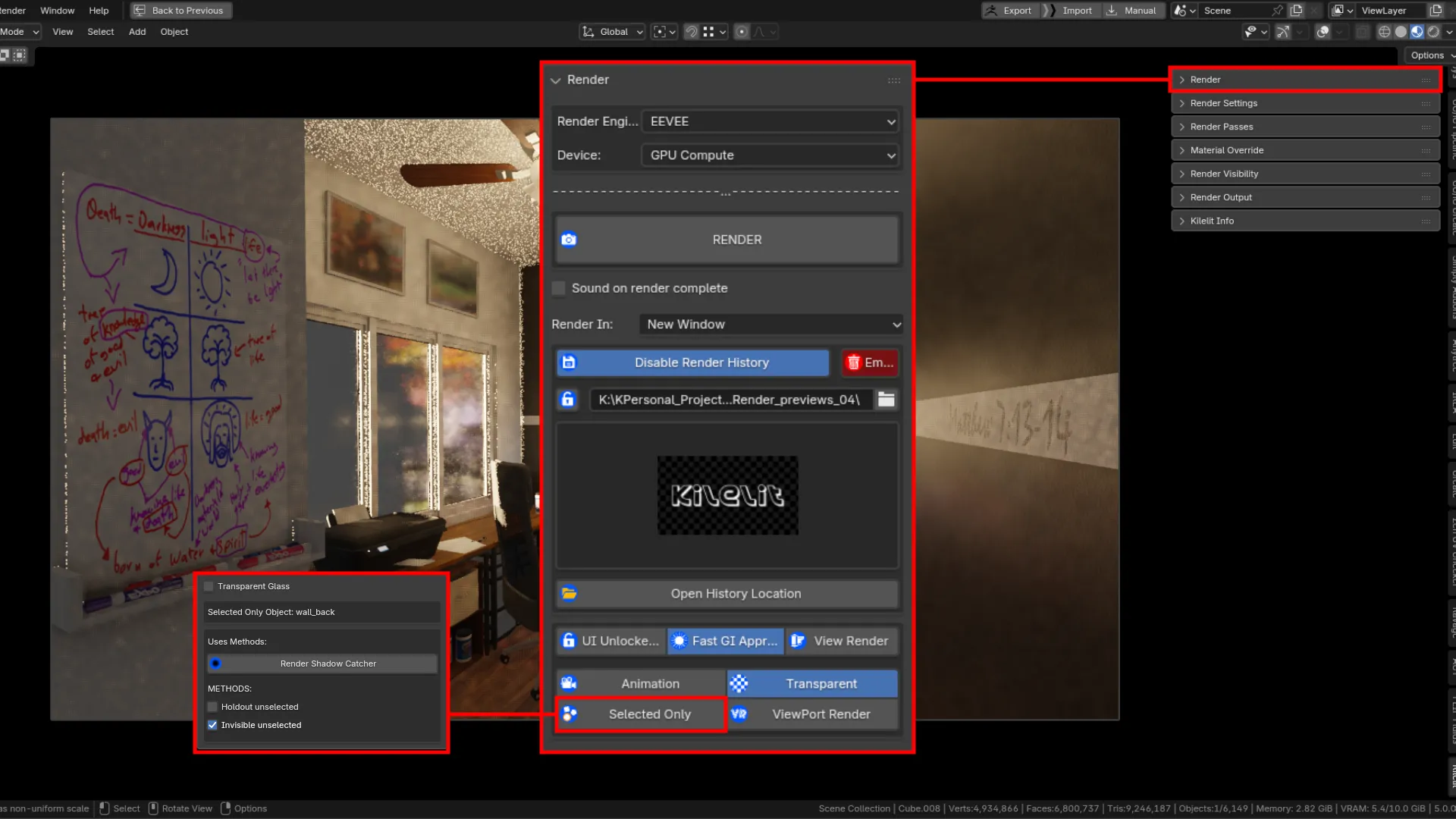
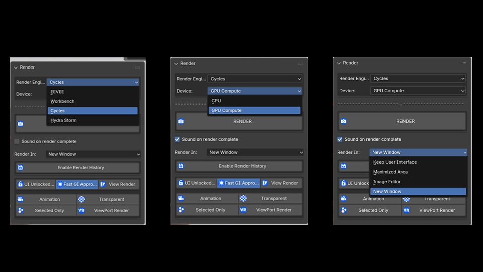
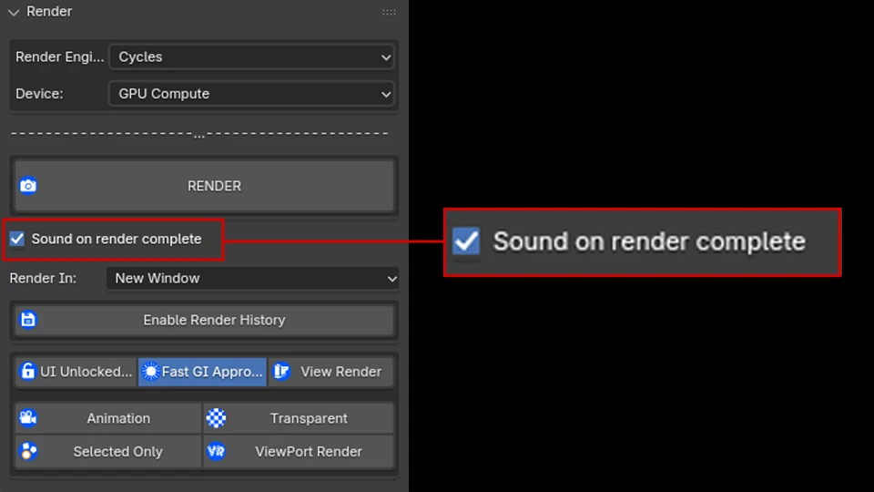
Included are built-in render settings such as the rollout selector for the [Render Engine] and what area of the ui you would like the render to occur. That includes !Image Editor, !New Window, !Maximum Area, or !Keep User Interface. Under the [Render] button, there is a checkbox for sound on render complete. This is a small, yet neat feature that makes a sound once a render is complete. This works for Cycles, Eevee, and viewport renders. Including still renders and/or animation renders. At this time, Kilelit is intended for Cycles, Eevee, and viewport render use.
Render History
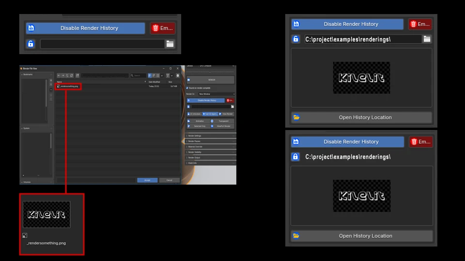
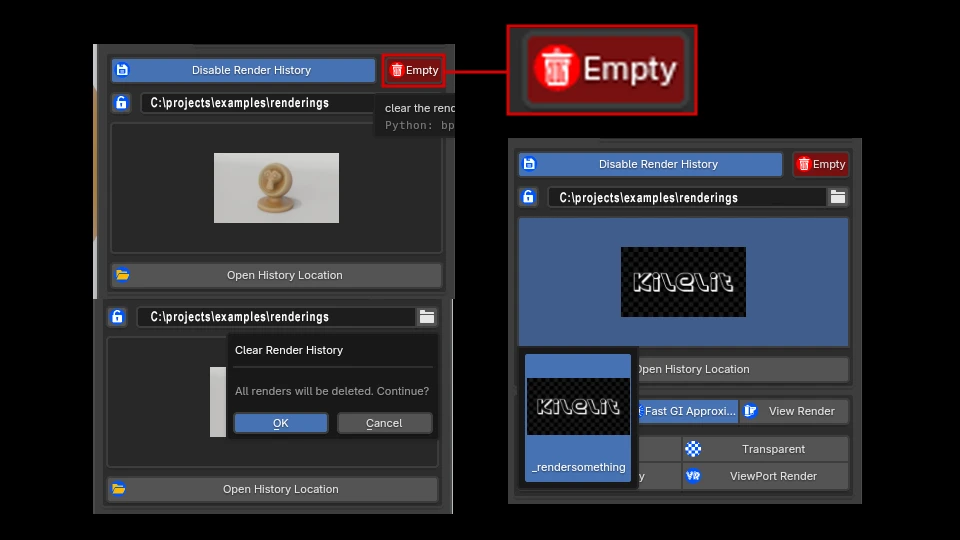
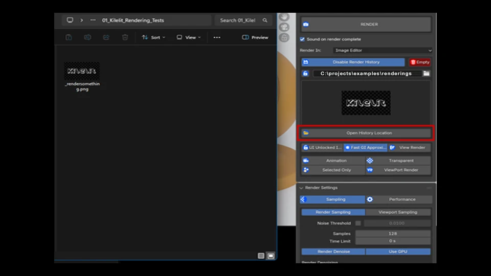
The first core feature to Kilelit/Ki is the [Render History]. This feature allows you to specify a directory you want your renders to be saved, and produce a render history throughout each iteration of renders you execute. This includes finished and canceled renders. Each iteration is automatically saved to the specified direction and named "kilelit_preview" post render. One important thing to note is that when you have the [Render History] enabled, the [UI Lock] will automatically be enabled at the start of the render and at the end of the render to ensure everything in the background finishes it's process before user interactions. This prevents errors occuring during render iteration auto saving. If you want to start with a clean slate, you can change the directory or click on the [Empty] button to the right of the history enable button. This will open a popup dialog with a warning. If you click on "Ok", the directory will be emptied. Deleting all the files named "kilelit_preview", except for the default image. Finally, if you would like to open the operating system's file explorer to the directory you specified, you can do that by click on the [Open History Location] button at the bottom of the previewer.
The [Render History] will be ignored when you have [Animation] mode toggled. Which we will cover within the next section of the !Render panel.
Rendering Modes
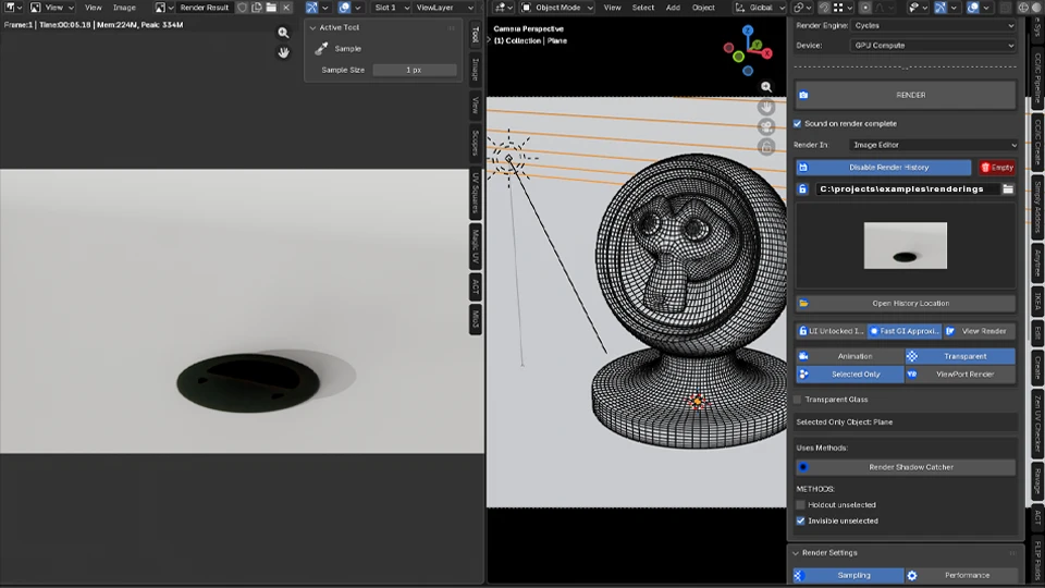
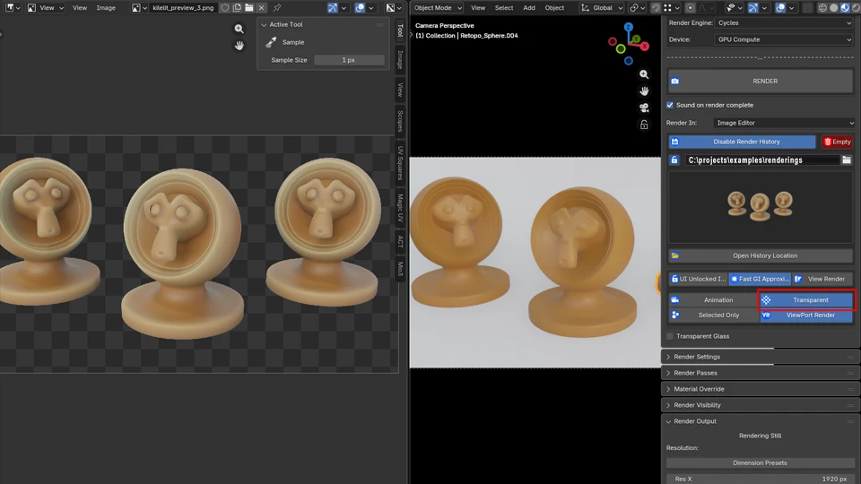
In the animation modes section of the !Render panel, we have three buttons at the upper level, and four at the bottom level. The three buttons at the top are placed here for specific scenarious, while also providing easy access to enabling a built-in feature. The [UI Lock Interface/Unlocked Interface], as the name suggest, will lock the interface during render. You will also see this toggle button enabled automatically when you render with the [Render History] feature enabled for reasons stated above. The [Fast GI Approximation] was added to this row, specifically for shadow catcher rendering scenarios. After some experimenting, I've noticed that with the Fast GI Approximation enabled, we can get a better shadow catcher render. The [Render Shadow Catcher] is located under the [Selected Only] render mode. Then we have the [View Render] button, which simply opens the !UV Editor or Image Editor area displaying the render results depending on which area you have selected in the !Render In rollout.
Animation Mode
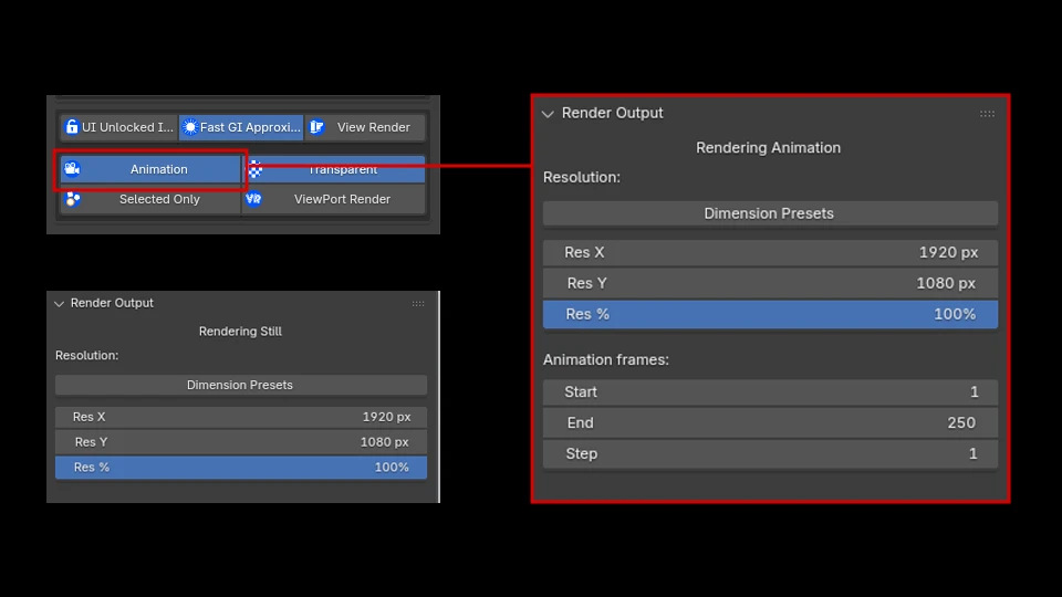
Now onto the last section of the !Render panel. Here we have our rendering modes, and they are pretty straight-forward and self-explanatory. The [Animation] mode will render an animation when you click on the [Render] button. When toggling this mode on, you will also see the timeframe range parameters show up inside the !Render Output panel. The [Animation] mode works with the [Selected Only] mode as well! You can render out an animation of the selected only object(s), which is very useful for compositing.
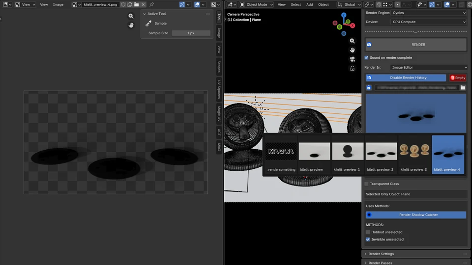
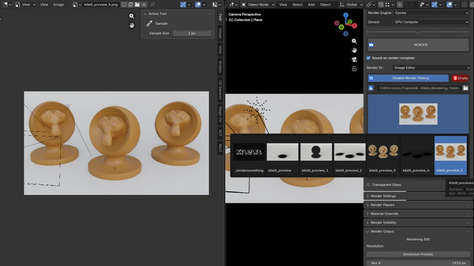
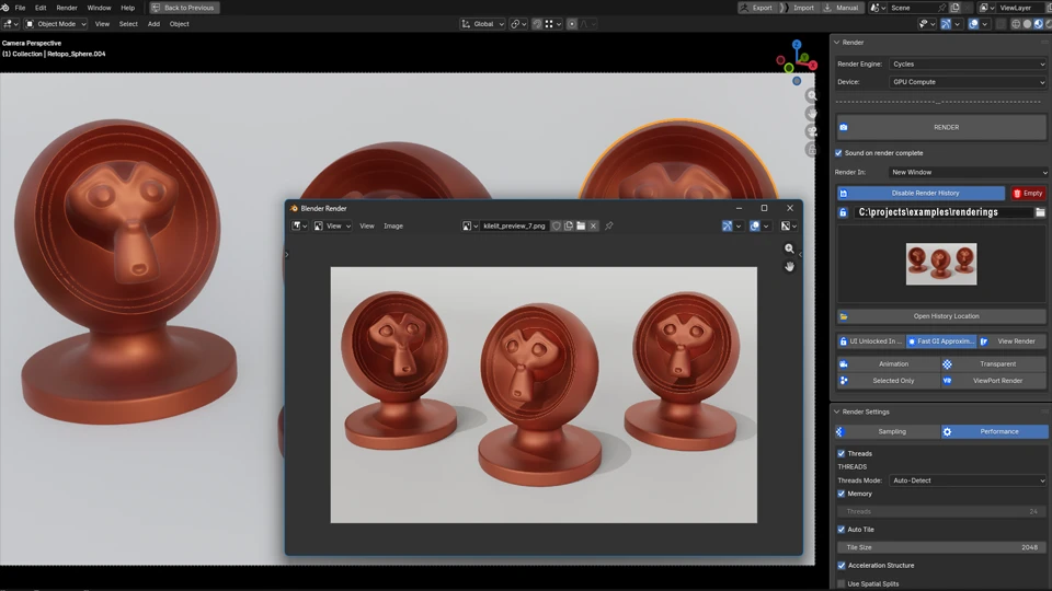
Selected Only Mode
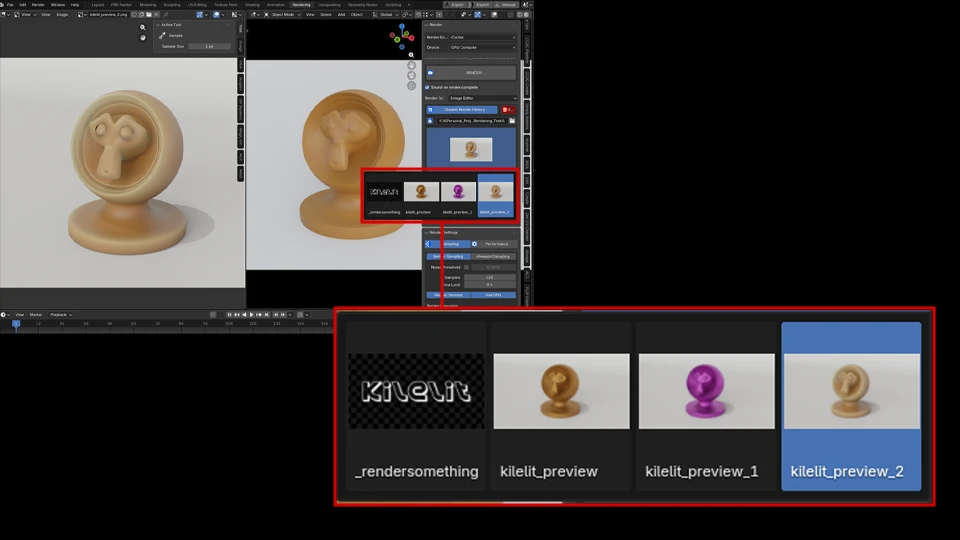
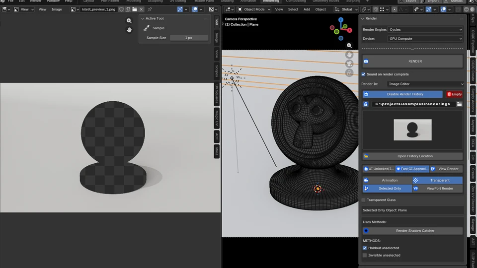
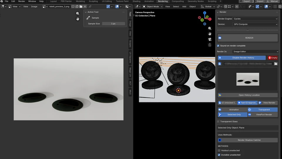
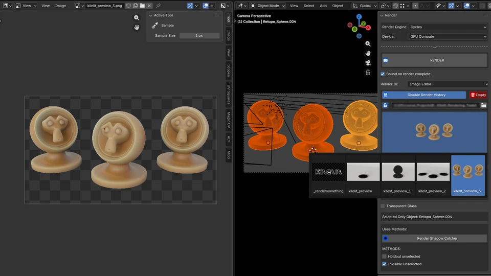
The second and third images showcase the different render selected only methods we can quickly generate with Kilelit. First the [Holdout unselected], then the [Invisible unselected] method. This works for multiple objects as well in both methods. Here we just have the floor object selected, and we can render the Suzanne Monkey Material models only as well. Shown in the fourth and fifth images. In the last image, you can also see the renders we have produced populating the history previewer, which we can cycle through selecting different renders to display in the !Image Editor area. The last feature here in the [Selected Only] mode is the [Render Shadow Catcher]. When toggled on, whatever object you have selected, it will render as a shadow catcher, and only rendering that selected object. This is very useful for producing shadow passes for product visualization or any post work(shown in the last image).
Viewport Render Mode & Wireframe Pass
The [ViewPort Render] mode will simply capture a screenshot of the viewport. Which is also compatible with the [Animation] mode. Blender has some really nice built-in viewport visualization and customization. This is extremely useful for setting up the viewport render for certain use cases. One case I use often is creating a wireframe pass by capturing the viewport. Whether still or animation, you can setup the Blender viewport to create a wireframe pass. You can do this by making sure you are in Solid mode, which you can enable by pressing +Z+ then selecting !Solid or pressing the +6+ key. Once there you want to open the !Viewport Shading drop-down menu then set the following:
!Lighting to [Flat].
!Wireframe Color to [Object] or [Theme] which you can set in the !Preferences -> !Themes -> !3D Viewport -> [Wire].
!Object Color to [Custom](Black)
!Background to [Custom](Black)
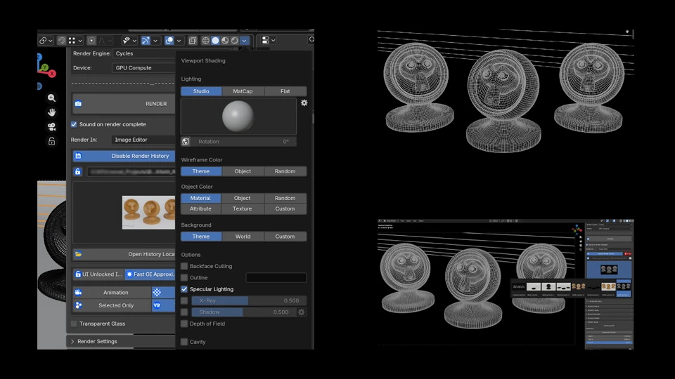
Finally, the [Transparent] enables Blender's [Film] property for transparent background.
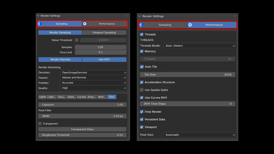
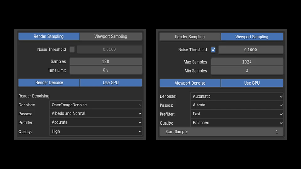
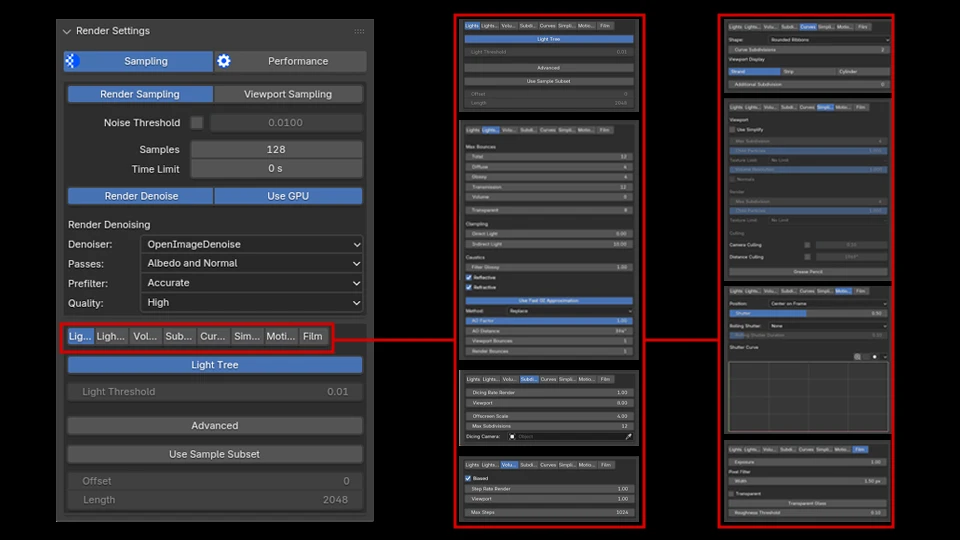
Render Settings
The second panel host man of Blender's built-in render settings. Giving the user access to the settings within Kilelit. On the top level, we have two tabs. The [Sampling] tab, and the [Performance] tab. The Ui will display whichever tab you enable, and they will switch respectively. The middle level, we have the sampling section. Including [Render Sampling] and [Viewport Sampling]. Which also determines the parameters to be displayed. These will also update respectively to each other, keeping the switch behavior. The bottom level includes many of the rendering parameters ranging from [Lights], [Lights Path], [Volumes], [Subdivision], [Curves], [Simplify], [Motion Blur], and [Film]. Addition parameters that deal more so with the performance side of things are located under the [Performance] tab. A unique take on the user-experience here is that these tabs are setup in a row structure and you can visit them one by one rather than scrolling up and down, which may be easier to look at.
This section does not replace the existing Blender render settings, but are built-in features added here so users can continue their rendering workflow while remaining within "Ki", if you will. A useful case for this idea is when you want to expand your viewport to focus on the scene look-dev. Of course you can customize your window, but this is a simple viewport expand with + Ctrl+SpaceBar +, and you will have many of the render parameters to work with still available.(Shown in fourth image)
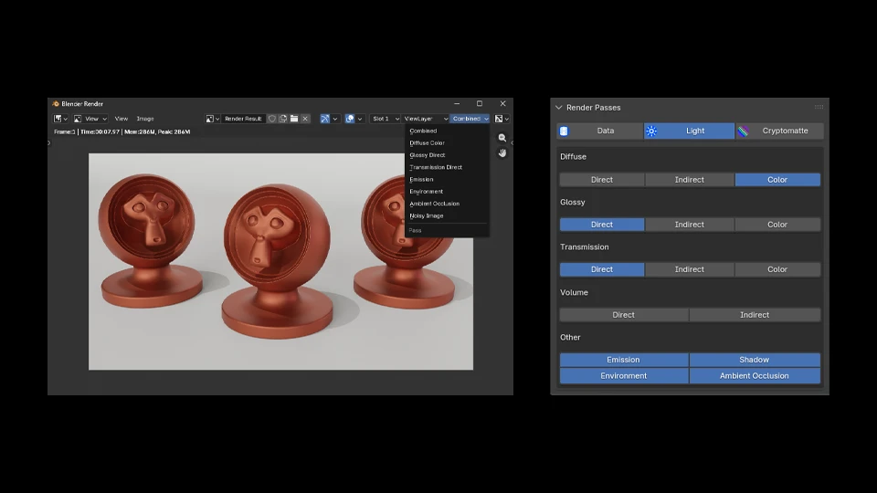
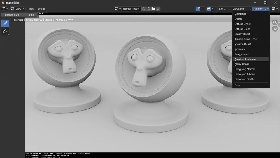
Render Passes
The third panel deals with !Render Passes. Here you can specify the pass you want included in your render. After a still render is complete, you can view these passes and export them separately for composition in post, or you can set your file format to exr and extract the passes in other DCCs that supports exr format. After the render is complete, !Render History will automatically set the latest render as the active image in the image editor. So you won't be able to see the passes drop-down menu here. If we switch the active image in the !Image Editor to the Render Results, we'll get the passes drop-down menu.
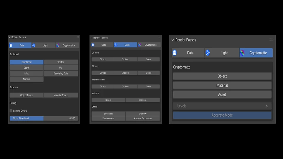
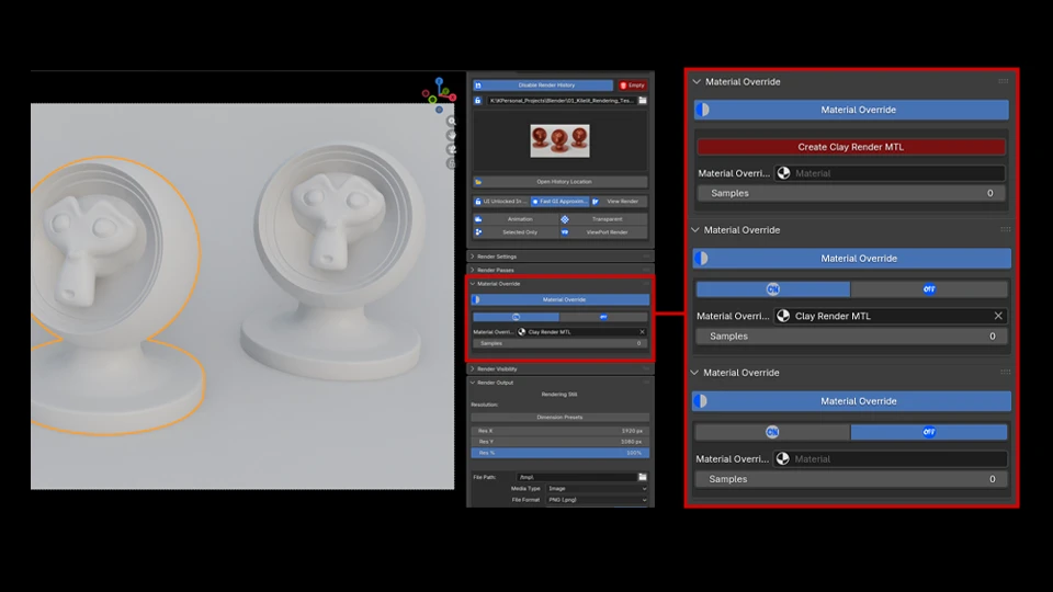
Material Override
The fourth panel is the !Material Override parameters, where we can simply click on Create Clay Render MTL, and that will create a material to globally override the scene. This is useful for a quick clay render setup.
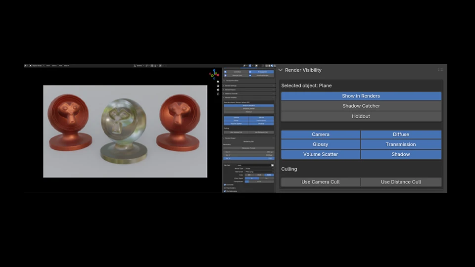
Render Visibility
The fifth panel here is the object visibility toggles. The only difference these parameters have in the way they function is you can adjust the visibility of multiple objects at once without the traditional Blender + alt+left-click + on buttons/toggles to affect all selected objects. However due proceed with caution how many objects you adjust at once as that can cause the scene to freeze. What it does in the background is it iterates through each selected object one at a time adjusting their visibility accordingly. This section works for both Cycles and Eevee.
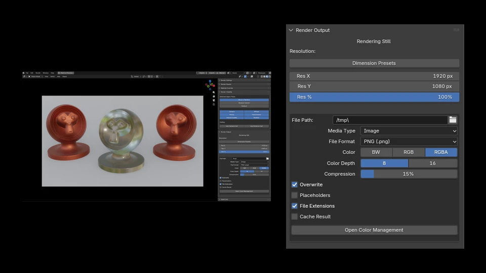
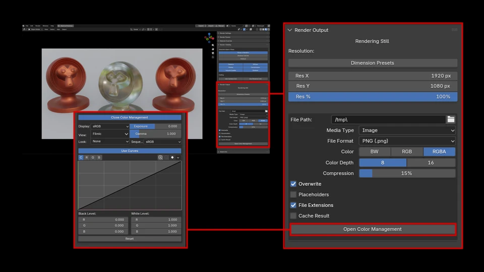
Render Output
The last panel for our rendering workflow is of course, the !Render Output. Here we can set our preferred settings for our output needs. As mentioned in the section regarding the head panel of Kilelit, !Render Panel, when you toggle animation mode, the output Ui will update where the timeline range is included.
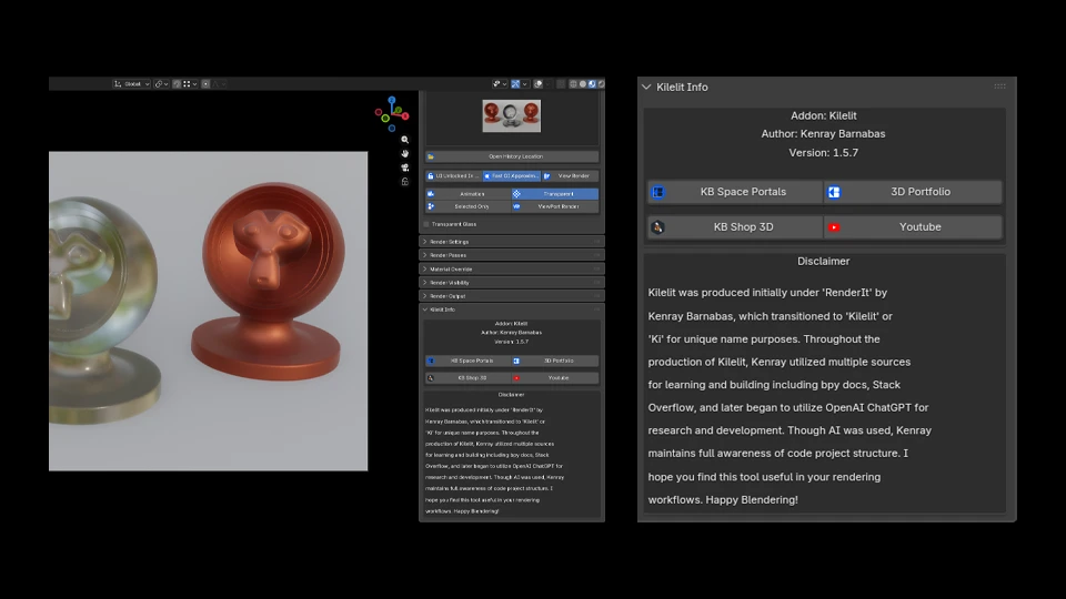
Kilelit Info
Last but not least, here you can find links to my platforms and the version of Kilelit you have installed. If you made it this far, thank you for visiting and checking out this add-on! I hope Kilelit proves useful in your rendering workflows.